Frequently Asked Questions
Frequently Asked Questions
Find our answers to frequently asked questions.
You have not found what you were looking for and you still have questions?
Please contact femfat.support.mpt(at)magna.com
In FEMFAT there are 3 options available for accelerating the analysis using "filters":
- Node filter: Only those nodes for which both the stress amplitude and the mean stress exceed a given value (% of the material endurance stress limit/tensile strength or absolute stress) are analyzed. That is, analyzed nodes do not suffer from a loss of precision, uncalculated nodes have no result (or dummy value). In BASIC the von Mises stress of the amplitude or mean stress tensor is used (see BASIC manual). In MAX differential stresses are adopted for certain critical times (see MAX manual).
- Cutting plane filter: In order to reduce the computation time when using the critical cutting plane method cutting planes can be filtered in MAX, i.e. they can be excluded a priori before the actual analysis. This can lead to a loss in precision. However, the filter is defined by default so that this very rarely needs attention. Three filter methods are available (see MAX manual).
- Rainflow amplitude limit: Load cycles with small amplitudes can be excluded in MAX, because they often only represent a very small proportion of the total damage. This can also affect a considerable acceleration in the analysis if the Rainflow matrix is dense at small amplitudes.
Further possibilities for reducing computation time include:
- Manual definition of a small analysis group (nodes + elements) –> no loss of precision.
- Reduction in Rainflow classes in MAX –> generally means loss of precision.
After a FEMFAT analysis, detailed local results (e.g. Haigh diagram, S/N curve, equivalent stress history for MAX) are output as standard for the critical node.
Due to boundary or contact conditions, it is possible that this node is not of interest to the user. This is why FEMFAT offers several possibilities for requesting this output for a specific node group.
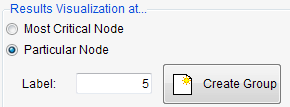
The first and simplest option is the targeted output for an individual node. This can be found in the FEMFAT menu “Analysis Parameters”, see Fig. 2. To do this, select the option “Particular Node” and enter the desired node label.
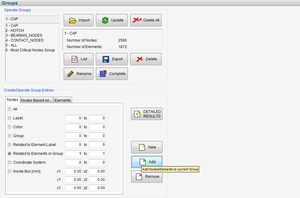
For several nodes, it is possible to request enhanced output via the “Detailed Results” group in FEMFAT. The definition can be made in the FEMFAT “Groups” menu as shown in Fig. 3, e.g. for a range of node labels. FEMFAT generates this group when the “Detailed Results” button is clicked.
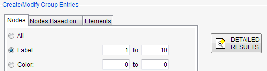
Attention: This group is not the analysis group because it only contains the nodes for the additional output.
Furthermore, detailed output items such as the local equivalent stress history or partial damage history are written to external ASCII files for the DETAILED RESULTS group in a MAX analysis.
These files can be imported into EXCEL, for example, and there be processed further. In addition, these data are also written to the fps file. Consequently, it is possible to display the local equivalent stress history in the VISUALIZER, for example.
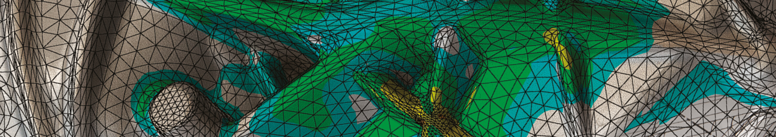
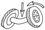
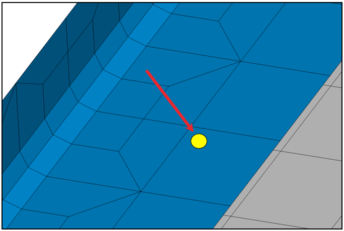
If for a FEMFAT design only a small part of the FE model is to be assessed or, if after a calculation has already been carried out the critical points are to be analyzed again with different parameters (different surface finish, different material, ...), it is important that in addition to the nodes to be evaluated all neighboring nodes and elements are also included in the new calculation group, so that the averaged element stress at nodes and the gradient calculation in FEMFAT can be performed correctly.
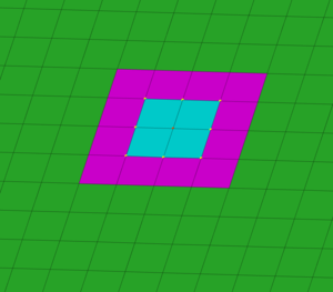
Fig. 1
If, for example, the red node (Fig. 1) is to be correctly calculated, the stress values of the adjacent elements have to be included in the group too for enabling a correct determination. The stress value at the FE nodes “connected via an element edge” must also be correctly determined (stress averaging) to enable correct determination of the relative stress gradients.
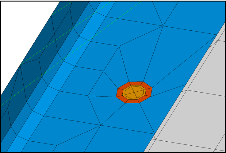
- Generate the group with the nodes to be considered.
- Enlarge the group by adding all elements connected to this node.
- Add all the nodes connected to these elements and the elements in turn connected to them to define the calculation group. If the node under consideration derives from a parabolic element, make sure that at least the adjacent corner nodes are also included in the calculation group (Fig. 2).
It is, of course, also possible to select a larger calculation group for a detailed area than that shown in the illustrations.
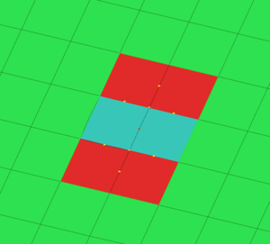
Fig. 2
Surrounding nodes and elements can be quickly and easily added in the FEMFAT group menu using the “Nodes/Elements related with Elements/Nodes from Group xx” option (Fig. 3).
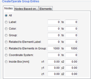
Fig. 3
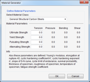
Only two items of basic information are required: the material group and the ultimate tensile strength of the material. It is possible to choose from 12 material groups in the material generator (10 iron and 2 aluminum material groups; see FKM guideline).
The material generator is based by default on the FKM guideline and generates material data for a survival probability of 97.5% for a specimen diameter of 7.5 mm.
After selection of the material group, the complete material dataset can be generated by entering the ultimate tensile strength.
An analysis can now be performed using such a dataset. It must be mentioned, however, that when using these material data, conservative results can be expected. The following data are advantageous in order to increase the precision:
- Tension/compression alternating strength σTA
- Tension/compression pulsating strength σTP (defined as upper stress in FEMFAT)
- Bending fatigue strength σBA
This makes it possible to find the mean stress sensitivity of the material using the relationship
M =2*σTA / σTP - 1
Furthermore, the support effect is defined by the ratio V= σBA / σTA (important for analyses with gradient influence in FEMFAT). The following steps apply if only one of the values mentioned is known:
- Determination of the values V and M of the base material.
- Modification of all values on the basis of, e.g. the known tension / compression alternating strength: σTA.
Example:
Material group, general structural carbon steels, UTS = 500 N/mm², Yield = 300 N/mm2, σTA = 250N/mm².
Step1: Selecting the material Group
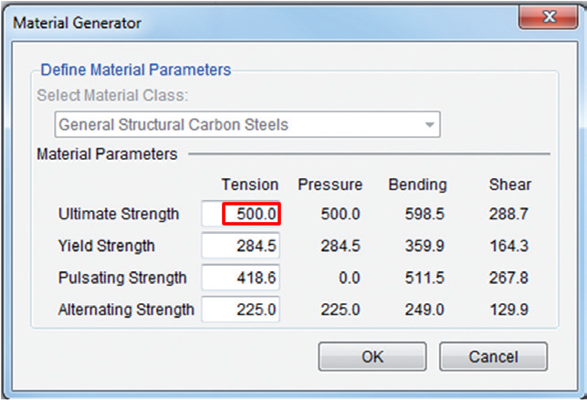
Figure 1
This influence stands for the determination of the local, static material properties, taking the stress gradient, isothermal temperature and technological parameter influences into consideration.
In the first step, the ductility for the "stress gradient" influence is estimated based on the elongation at rupture of the material (see Fig. 1), which subsequently determines the maximum achievable value of the local ultimate stress limit.

Figure 1

Figure 2
In the next step, the corresponding ultimate stress value is calculated based on the known tensile strength (rel. gradient = 0), the ultimate bending stress (rel. gradient = 2/specimen thickness) and the previously determined relative stress gradient (see Fig. 2). The "limit line" (red) is given by the factor from the first step.
The ultimate stress is reduced in analogy to the equations in the FKM guideline for the isothermal temperature influence (default method "FEMFAT 4.6"). If a user-defined temperature influence is used, FEMFAT uses the corresponding polygon from the material definition (temperature -> strength reduction to ultimate stress).
Moreover, the technological size influence can additionally be taken into consideration for large wall thicknesses/diameters; it is also taken into consideration in accordance with the FKM Guideline.
The analysis group can be freely defined by the user, either in the preprocessor (I-DEAS, MEDINA, PATRAN, etc.) or with the help of FEMFAT.
FEMFAT gives analysis results for FE-nodes only but needs the surrounding elements for their stress data and the accurate stress at adjacent FE-nodes which makes the necessary data for an analysis tremendously larger than just a few FE-nodes. To analyze one FE-node FEMFAT takes the stress gradient into account, why the accurate nodal stress (averaged from their adjacent elements) of all surrounding FE-nodes in direct connection are needed.
The user can make the necessary group extension in a few steps. It is advisable to first create a copy of the corresponding group. Then, by using the group function "Add elements related to nodes in group," the user adds the neighboring elements.
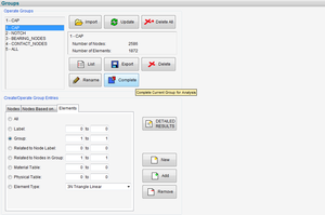
The automatic „one click solution“ is the button “Complete”(for Analysis) which does pretty much the same than the three clicks from manual solution.

If this new group is selected for the analysis, the result at FE nodes in the original group (which has been copied at the beginning) is correct.
If several groups have been defined, e.g. for the definition of the surface roughness, temperatures and so on, it has to be considered that before the start of the FEMFAT calculation or the generation of the MAX scratch files, the correct calculation group has to be activated. This can be checked very easily by “CHECK INPUT DATA”, because the active group for calculation is mentioned there again.
To speed up the FEMFAT analysis the user can define a stress amplitude filter. There are two possibilities:
- relative stress amplitude filter [%]
- absolute stress amplitude filter [MPa]
For the relative stress amplitude filter FEMFAT needs a percent value, which is related to the material alternating endurance limit (tension). By default, the relative stress filter is 40%, then all nodes will be analyzed for which the amplitude stress is higher than 40% of the material endurance limit (alternating strength for tension) and the mean stress is bigger than 40% of the UTS. For the absolute stress amplitude limit the user directly types in the stress limit [MPa].
For example the user chooses 30 MPa, all nodes having a lower stress amplitude than 30 MPa will be filtered. Therefore take care, if there is a very high mean stress and small amplitude stress at nodes. In such case we recommend to switch to the absolute amplitude stress limit.


FEMFAT basic
for proportional loading that can be described by two states and a constant component (e.g. assembly).
Advantage: the analysis speed is very fast because FEMFAT basic holds the data in RAM.
Examples: Conrod, cylinder head, gearbox casing, shafts etc.
Input data required:
- Upper/lower stress or amplitude/mean stress
- Constant stress (optional)
- Load spectrum for damage analysis

ChannelMAX
The loading consits of stresses due to unit load cases and the corresponding load-histories. The system response (except local plastic deformations) must be linear because of the linear superposition of the unit load cases.
Examples: wheel mounts, axle frames, body work, crank shafts
Input data required:
- One stress result per channel (load direction, modal shape)
- One load-time sequence per channel
TransMAX
Most general form of the load history. The system response can be completely non-linear; number of time points limited to hundreds (thousands).
Examples: cylinder block and other components with complex contacts.
Input data required:
- Sequence of computed stress states over time
Six equivalent stresses are available in FEMFAT basic, in MAX this increases to 11 equivalent stresses. Generally speaking, the user need not be concerned with selection of the correct equivalent stress. The BASIC and MAX modules use the "Automatic" default setting. This is recommended by the ECS for all cases. Using this setting, the equivalent stress adopted is decided on the basis of the local material at the respective node. If a (brittle) gray cast iron is being dealt with, both BASIC and MAX employ the normal-stress hypothesis in conjunction with the critical cutting plane method.
If calculations are performed in FEMFAT MAX using the default "Automatic" setting, a scaled normal stress is formed in the cutting plane for all materials with the exception of gray cast iron. The use of a scaled normal stress solves what is known as the "sign problem", which may occur with most other equivalent stresses provided in FEMFAT MAX but which are now no longer recommended. The sign is required to form an equivalent stress history, in order to take both tensile and compressive stresses into consideration. However, this can lead to unphysical leaps in the equivalent stress history for non-proportional loading, depending on the selected equivalent stress, and thus to inexact and highly conservative damage results.
A special advantage of automatic selection is the possibility of combining a variety of materials during a single analysis run.
The scaled normal stress offers a procedure that eradicates this problem and that works just as efficiently as the "simple" normal stress without scaling. By applying a scaling factor to the normal stress the material ductility (brittle/semi-ductile/ductile) and the type of loading (tension-compression/bending, shear/torsion, hydrostatic stress state) can be incorporated in the analysis and be adequately considered even for non-proportional loading. A particular advantage of this scaled normal stress also lies in the fact that the triaxial stress states within the component or at compression-loaded component surfaces can be easily evaluated. The generally minor damaging effects of hydrostatic stress states are correctly modeled.
The use of invariants (von Mises' and max./min. principle stresses), on the other hand, does not allow consideration of arbitrary material ratios. We therefore no longer recommend the use of these equivalent stresses. They are still provided for historical reasons.
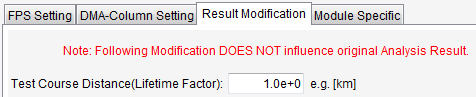
If these are only minor differences they may be the result of rounding errors in the protocol file (4 decimal places) or the visualization in your postprocessor. A further possibility is the use of the test track length input in "Output modification" (see below). These modifications only apply to the dma file, the factor is not calculated for the protocol file.
The Result Manager provides options for better result visualization of FEMFAT results. For example, it is possible to perform a minimum/maximum search of several FEMFAT results. Additionally, an equation editor is available beside the simple linear combination option for individual results. The damage results can be merged here by way of user-defined equations. This allows simple computation of the utilization factor of welds according to the FKM guideline, for example. The result is immediately available to VISUALIZER in the fps file or can be exported in the usual result formats.
In some loading situations, e.g. in crankshafts subject to combined bending/torsional loads, a local change or rotation in the directions of the principal stresses may occur with time.
Tests using combined bending/torsional alternating loads and 90 degree phase shift have shown that for ductile materials (tempered steel) the critical cutting plane method overestimates the lifetime (e.g. see FKM report "Multiaxial Fatigue Analysis, 2002"). In FEMFAT max it is possible to correlate the lifetime using "Influence of rotating principal stresses".
The local S/N curve is reduced as a function of a statistical degree of multiaxiality lying between 0 (= proportional load with constant direction of principal stresses) and 1 (= heavily nonproportional load with directions of principal stresses changeable with time).
The influence thus results in a reduction in lifetime in ductile materials. No impact is defined for brittle cast materials (gray cast iron, cast Al, cast Mg).
We recommend activating the influence of rotating principal stresses. However, in certain cases, e.g. where high constant stresses are involved (bolt pre-stresses, residual stresses), the results may be conservative.
The Batch Job feature is intended to allow FEMFAT to run in the background automatically with no interactive input on the user interface. It is especially helpful to use batch jobs when a number of FEMFAT analyses must be carried out (e.g. engine run-up). Typically, a FEMFAT job in the batch mode is invoked
using the following call:
- …/bin/femfat –job=jobfilename (Linux)
- …/bin/femfat.bat –job=jobfilename (Windows)
This standard call can be expanded using additional Parameters which offer the user a wide range of possibilities. For example, it is possible to specify a separate scratch Directory for the individual jobs,
- …/bin/femfat –job=jobfilename -scr=Scratch_Directory (Linux)
- …/bin/femfat.bat –job=jobfilename -scr=Scratch_Directory (Windows)
or disable individual modules (here: PLAST):
- …/bin/femfat –job=jobfilename -noplast (Linux)
- …/bin/femfat.bat –job=jobfilename –noplast (Windows)
A detailed overview of all available parameters can be found in the “FEMFAT_Introduction.pdf” manual. This manual is contained in the installation directory in both German and English along with all the other module manuals.
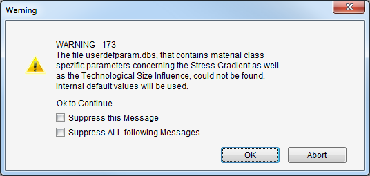
The background for this message is that during the Definition of the new working directory in the ini file, a path was selected for the material import which does not contain the userdefparam. dbs file. This database makes it possible to adapt fundamental properties which are material-class specific (slope exponent of S/N curve, material-dependent exponent, exponents for gradient influence, etc.). If you have not made any modifications in the database, then you can ignore this message and click “OK”. In this case, FEMFAT uses the database with the respective default values from the installation directory. If you have modified the userdefparam.dbs file and wish to use it, then you must either copy the database to the specific working directory or change the default import path for materials in the FEMFAT settings to reflect the corresponding save location.
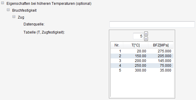
In many applications, elevated temperatures occur. In order to take these into account in the fatigue analysis, the isothermal temperature must first be specified in the node characteristics menu, either as constant value or as temperature distribution from FEA. In the next step, the influence factor „Isothermal temperature influence“ has to be activated.
By default, the strength values are then reduced according to the „FEMFAT 4.6“ method based on the FKM guideline.
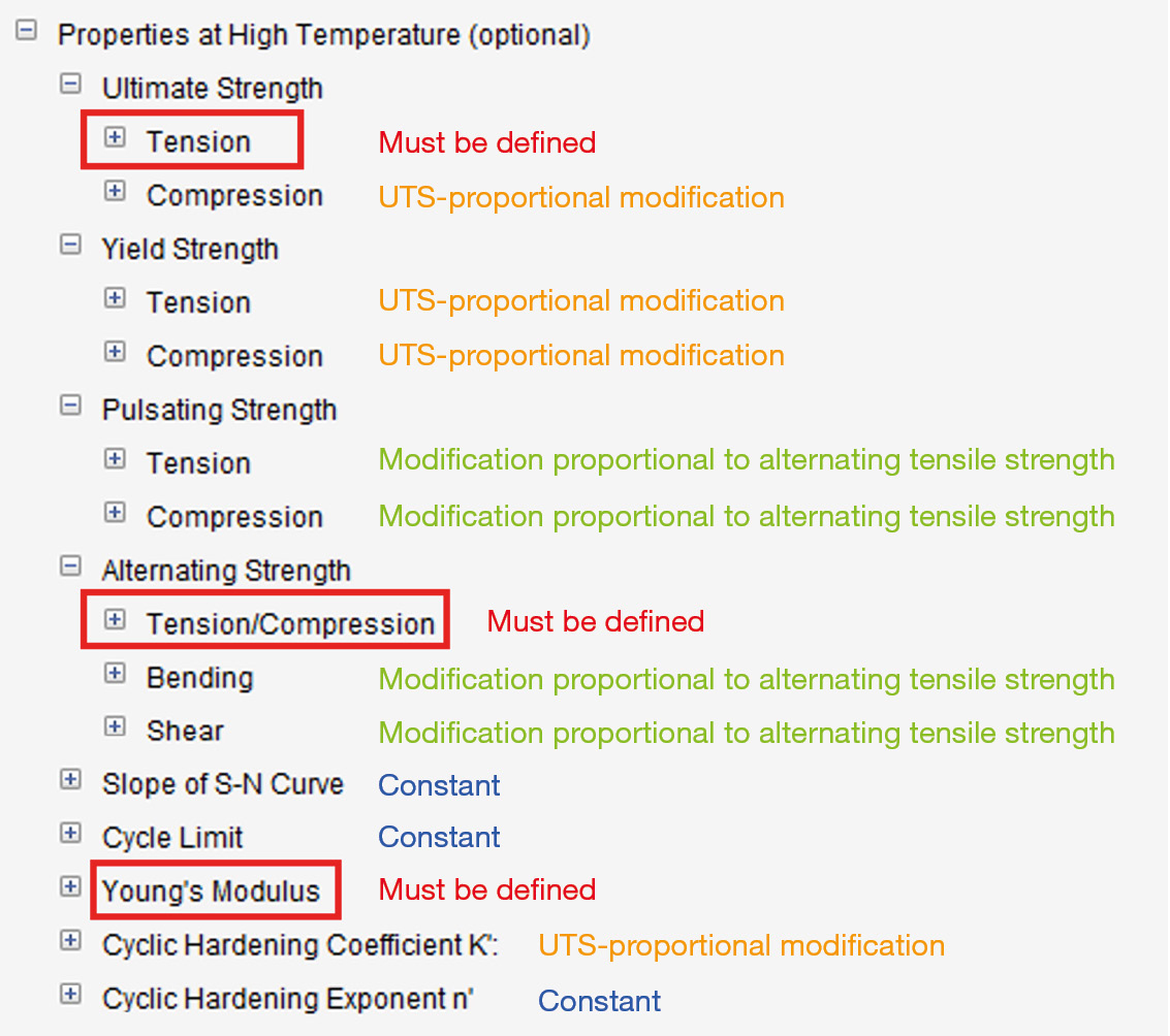
In addition, FEMFAT offers the possibility to specify the material behavior at higher temperatures. The temperature-dependent behavior can be specified not only for the static and dynamic strength values but also for the S/N curve parameters, the Young‘s modulus and the cyclic hardening coefficient or exponent.
However, despite all flexibility, it should be noted that not all of these input options are mandatory. The minimum requirement for using the user-defined temperature influence is the specification of the temperature-dependent values for the Young‘s modulus as well as ultimate tensile strength and alternating tensile / compressive strength. The remaining strength data are then – if not specified – automatically reduced proportionally to these values or kept constant, cp. also the following picture.
FAQ 1: Treatment of the stresses of parabolic elements from ANSYS * .rst in FEMFAT
In the ANSYS * .rst file, no node-related results (stresses, strains, ...) are saved for the middle nodes of finite elements with parabolic shape functions. So that an analysis of these middle nodes can still be carried out in FEMFAT, the results of the adjacent corner nodes are used to determine values for middle nodes.
For stresses this is done as follows:
- In the first step, the stress tensor at the center nodes is calculated component wise by arithmetic averaging of the stress tensor at the associated corner nodes. This is done immediately after reading the stresses in FEMFAT for each element with element node stresses. As a result, element node stresses are again obtained at the middle node, i.e. if the middle node belongs to several elements, the stress tensor differs from element to element.
- In the second step, FEMFAT requires node-averaged stresses for the base material calculation. These are determined either when the calculation starts (BASIC), when the VISUALIZER is started in the stress data dialog (BASIC) or when scratching (MAX, HEAT, SPECTRAL). The mean stress tensors of each element at the central node are again arithmetically averaged component by component and the node-averaged stresses are obtained for the FEMFAT calculation:

The analogous procedure applies for strains in HEAT. For node results, such as temperatures, the middle node values are read directly from the rst file.

The default settings regarding influence factors and analysis parameters reflect our recommendations for the fatigue analysis. To follow your own “guidelines” in the department or in the group, you sometimes have to overwrite these defaults.
We provided the first help with the templates in FEMFAT 5.1 (2014). They can be found in the FEMFAT installation directory / templates and include the weld sensitivity analysis, the recommended settings for GL 2010 and the evaluation of elastomers.
Calling and reading job files is easy with the icon on the graphical user interface , but as such is not recorded in the ffj file. Instead, the read lines are appended to the current job file.
In the batch job such a call has to be inserted with the TCL / TK command "source" (the absolut path must be specified or a variable previously defined in the program must be used, as here "installation_path"):
source $installation_path/templates/WELD_Sensitivity_Damage_gap.ffj
The previously described use of variables with the "set" command to assign the "installation_path" the standard installation directory of FEMFAT 5.4 then looks like this:
set installation_path „C:/Program Files/ECS/FEMFAT5.4“
If a job in which another job was read is saved after this action, it is no longer the call of the template or the job that is saved, but the lines from the template! So you have to decide whether you want to keep / save the calculated job files or the previously prepared job file or both.
Other TCL / TK commands that make it easier for you to design your jobs with FEMFAT can also be found in the templates for the WELD sensitivity analysis.
However, we would like to point out again that manually edited job files are not the standard and can only be examined by our support with additional effort.
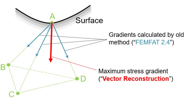
FEMFAT so far used to calculate the stress gradient along the finite element edges by considering the stress gradient between two neighbouring nodes.
In most cases, the maximum stress gradient is perpendicular to the surface. Since parabolic tetrahedron elements are typically used in the meshing of a complex shaped structure, there are often no finite element edges perpendicular to the surface. This can lead to less accurate results.
The new method ("Vector Reconstruction") uses the stress gradients along the finite element edges to reconstruct the maximum stress gradient. This is done independently of whether there is an element edge in this direction or not.
Note: this new method is the default setting for BASIC, TransMAX and SPECTRAL as of FEMFAT 2022.
ChannelMAX has two special features in this respect: firstly, the method "Vector reconstruction reduced" is used as default. Thereby not all samples of the load-time curves are used, but only those at which minimum and maximum occur in the respective load time histories of the channels. Furthermore, in ChannelMAX, if a "Vector Reconstruction" method is selected, additionally the gradient is formed analog to TransMAX based on the superposed, time-dependent stress tensors.
If FEMFAT job files (*.ffj) older than v2022 are used, the old gradient method "FEMFAT 2.4" is automatically activated.
The data relevant for FEMFAT are read from an odb file with the libraries supplied by Dassault and the FEMFAT application feadapter.exe.
The feadapter and the corresponding libraries are of course dependent on the respective odb version. Also, files of older versions can be read in principle. However, these had to be updated to this version before - a process that takes additional time if the interface installed in FEMFAT does not exactly match the Abaqus version used.
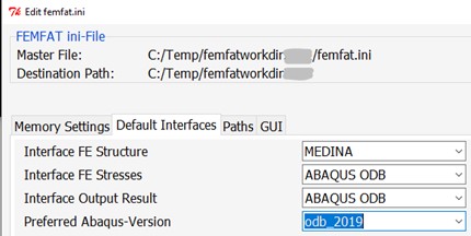
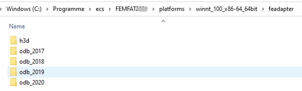
Since FEMFAT 5.4.1 the program behavior has been improved significantly. FEMFAT includes now several odb interfaces. In the configuration file femfat.ini in the working directory the user can define his preferred ABAQUS version. In the selection box all folders starting with "odb_" are listed and are ranked lexicographically.
When reading an odb file, FEMFAT first searches for the suitable library version before starting the update process. If FEMFAT finds a suitable library, the file is read without any loss of time. If no matching library is found and the odb version is older than the versions installed in FEMFAT, an update is written to a new file using the default Abaqus version and the original filename is suffixed with "_upd". The new file is in the working directory, along with the feadapter.log file for details on the import process.
Conversely, if the standard interface notices that the odb file is "too new" and no newer odb libraries are found, an error message is issued that the odb file cannot be read.
Newer odb libraries are available on the FEMFAT homepage www.femfat.com . After the download, place the unzipped folder in the following directory
FEMFATINSTALLATIONPATH/platforms/<Win oder linux>/feadapter/
What Options Do I Have for Efficient Analysis and Evaluation of Base Material, SPOT, and WELD Nodes?
When performing durability analysis on large FE structures, computation times can be lengthy.
A practical way to keep computation times low, is to define an analysis filter in the “Analysis Parameters” menu. This filter excludes nodes whose maximum amplitude and mean stress are below a certain threshold, ensuring that only structurally significant areas are evaluated.
For efficient analysis, you can set individual filter values for base material, SPOT, WELD, and LAMINATE calculations by activating the "Advanced" checkbox. Additionally, a similar filter function is available for output in the *.pro protocol file.
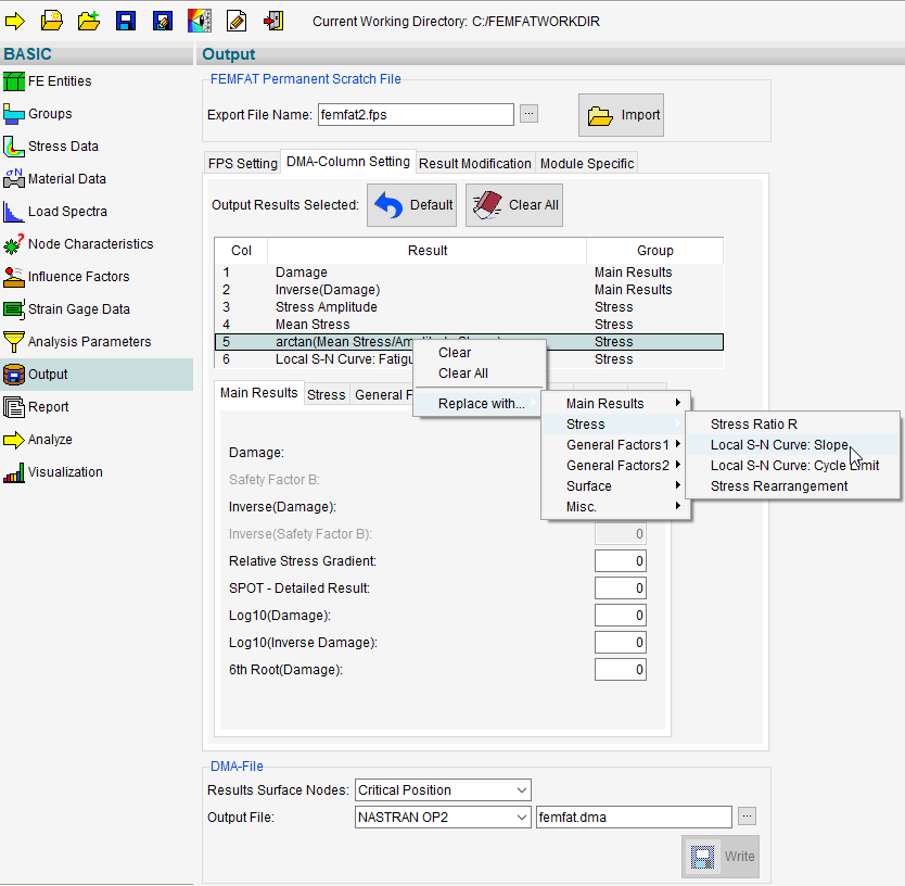
For dma files in NASTRAN OP2 and ABAQUS ODB formats, FEMFAT results for base material (including laminates) and WELD and SPOT nodes can be output into separate datasets. This separation simplifies the visualization and evaluation of connection technology results from the base material in the post-processor.
FEMFAT provides the user with a variety of options for checking input during analysis preparation or following the analysis. These are:
FEM-Model
- Number of imported nodes & elements (Caution: some "exotic" element types are ignored).
- Dimensions of model (unit correction to mm may be necessary)
- Minimum/maximum shell thicknesses
- Visual control in VISUALIZER including group definition; groups can be displayed in the main program as a label list.
Material Data
- Numerical control of the data in the material menu
- Graphical control using the Haigh diagram, S/N curve and cyclic σ - ε diagram
- In the node characteristics menu by browsing in the node labels for checking all properties (material, roughness, temperature, surface treatment,...)
Stresses
- In BASIC maximum principle stress of the element with the highest v. Mises equivalent stress
- For MAX, visual control of the stress sequence or the unit stresses is available in the VISUALIZER.
Menu Item "Check Input Data"
This function is available immediately prior to starting the analysis that allows a number of input data to be double-checked, in particular, whether the stresses and the material strength form a plausible relationship in terms of the required analysis result (endurance safety factor, damage life in the finite life domain, static safety). Implementation of these checks is strongly recommended, see figure below.

Note:
Execution of this function may take some time in MAX, especially if the scratch files have not yet been created.
The following data can be examined in detail:
- Analysis aim: Endurance, damage, static safety .
- Analysis group: Name and number of nodes and elements
- Materials used in the analysis group, including data plausibility check
- Activated influence parameters
- Stresses
- Maximum occurring v. Mises stress for the entire load history compared to the local tensile strength/yield stress.
- Maximum v. Mises stresses of individual load channels (ChannelMAX only). This function is very useful for estimating the influence of certain channels on the overall result. For example, using the modal superposition method a frequency boundary can be defined in this way above which the higher frequency modes need not be taken into consideration due to the small stress value.
Because the load-time histories and the channel stresses are combined for this function, inconsistent units can also be easily discovered.
Results
- Result dialog: Maximum stressed node, S/N curve, utilization statistics.
- Distribution of all scalar result variables on the model: Any postprocessor can be employed for this or, most comfortably, the VISUALIZER.
Documentation
Up until the release of version 5.1, the FEMFAT license module retrieved all the necessary and available licenses from the license server unless other settings had been specified manually. Since the release of FEMFAT 5.1, individual licenses are only retrieved while the server is being used and they are made available again during times of non-use. In this regard, it is also possible to specify a timeout which defines the time interval of the users inactivity after which the license is once again made available. This has the advantage that other users can use the licenses and therefore, no valuable resources remain unused. The default value for the timeout is 15 minutes. The “MAGNAECS_LICENSE_TIMEOUT” environment variable allows a value of between 5 and 9999 minutes to be set. If work with FEMFAT is resumed after the timeout value was exceeded, FEMFAT attempts to retrieve the required licenses once again. If they have already been reassigned, then there are the options of either waiting until a license becomes available or of saving the state of the model temporarily and continuing work at a later point in time. However, FEMFAT will be exited either way. For analyses which are carried out in batch mode, the keyword “-queue” can be used to prevent FEMFAT from aborting the job due to a lack of licenses and writing an entry into the message file. Instead, FEMFAT then waits with the further processing until a sufficient number of licenses are available. This means that, overall, variable licensing provides significant improvements: Licenses are only blocked as long as they are actually required for an analysis. This increases the utilization capacity of the existing licenses when there are several analysis engineers working with one license pool.
Before you begin, make sure you have the following resources:
- Sufficient Hard Disk and Main Memory: The FEMFAT installation currently (FEMFAT 5.3) requires about 500MB hard disk space. Additional space should be provided for (result) files generated during the FEMFAT analysis. For the application itself at least 4GB RAM main memory are to be planned.
- Installation Package for License Management Software (“License Server”): Currently the management of the FEMFAT licenses is done with the software LM-X of X-Formation. The required installation package can be found both in the FEMFAT installation, e.g. under .../femfat53/platforms/winnt_61_x86-64_64bit/lmx as well as a separate download on our homepage. Please note that the software downloads are only available to registered users with corresponding user rights!
- A valid License File: The generation of a license file requires hardware information from the computer on which the license server will later be installed. In the installation package of the license server you will find the application “lmxendutil”. Execute these on the appropriate computer. Please send the generated output to FEMFAT Support ( femfat.support.mpt(at)magna.com ) for the license file creation.
- FEMFAT Installation Package: It is available in the download area on our homepage.
To use FEMFAT proceed as follows:
- Installation of the License Server: The installation is carried out on the machine which is to manage the license requests of the users ("clients"). The corresponding installation package contains a file for the automatic setup of the license server as a Windows service or as Demon on UNIX. This step can be skipped for a local (uncounted node-locked) license.
- Configuration of the License Server (editing the file “magnaecs.cfg“): By modifying the file "magnaecs.cfg" you configure the license server by specifying the log and license file, the port to be used etc...
- Start the License Server
- Installation of the FEMFAT Software on the Client
- Definition of a new Environment Variable "MAGNAECS_LICENSE_PATH" on the Client: The value of this environment variable is - port@servername in the case of a network license ("floating" license) or - the complete path of the license file in case of an "uncounted node-locked" license.
FEMFAT is now available on the client machine.
With Windows 10, Microsoft has changed their release strategy: so-called Feature Updates will replace the previous releases of new Windows versions at a frequency of about 3-5 years. These Feature Updates will be released twice per year. Microsoft envisions “Servicing Channels” which are designed to give customers a certain amount of control with respect to the point of time for updates. These allow the function update to be carried out twice per year (“Semi-Annual Channel”) or about every 3 years (“Long-Term Servicing Channel”). The FEMFAT platform strategy will be adapted to this new situation so that both the “Semi-Annual Channel” and the “Long-Term Servicing Channel” are supported. Specifically, this means that if Windows 10 Feature Updates restrict the proper execution of FEMFAT, executable installation packages will be supplied for the most current versions of the last two major releases (e.g. FEMFAT 5.4 and FEMFAT 5.3) within a reasonable period of time (additional information on the tested operating system updates will be provided shortly on our website.)
The result of the fatigue analysis is strongly influenced by the quality of the material data. Unfortunately, during the development process, there is hardly any chance to know all material values, therefore there is the possibility in FEMFAT to generate a new material based on only few data.
This support, offered by FEMFAT, is based on certain materials laws, specific for each material class (e.g. aluminum casting alloys, gray cast iron,...). It is very important to activate the correct material class before generating the new material. Please check the Haigh diagram after using the material generator, because possible failures can there be seen very easily.
If you need help for generation of new materials, please do not hesitate to contact the FEMFAT support at femfat.support.mpt(at)magna.com
Today’s commercial simulation tools provide the possibility of simulating the casting process and of predicting the associated inhomogeneous structure conditions within the component. This gives, amongst other things, a distribution of the secondary dendrite arm spacing (SDAS), the solidification time, the cooling rate or the microporosity. It is possible to import these distributions into FEMFAT and to consider their influence on the endurance stress limit. Here, the solidification time and the cooling rate can be converted to an SDAS by means of an exponential approach. The currently implemented dependence of the endurance stress limit on the SDAS is optimized for aluminum sand and gravity die casting. However, the influence of the SDAS on the endurance stress limit can, if known, also be given by the user as a value pair table for any material. A new material dataset with the number 220 was created for this purpose. Nevertheless, it is also possible to consider microporosities or other structural parameters. In FEMFAT, the distribution of any structural parameter can be imported via the same interface, instead of an SDAS distribution. The only requirement is that the values are node-referenced. The file format thus corresponds to (node-referenced) temperature data. Moreover, for an operational strength evaluation, the influence of the specified structural parameter on the material endurance stress limit must be known and be defined by means of a table (dataset 220) in the material file (*.ffd).
The influence of cast structure in FEMFAT is already being successfully implemented by BMW in their engine development process, e.g. for cylinder heads.

S/N curves for varying SDAS

Effects of SDAS on the analysed endurance safety factors*
*[P. Nefischer, F. Steinparzer, H. Kratochwill, G. Steinwänder, BMW Motoren GmbH; "New approaches in damage analysis of cylinder heads" (New approaches in damage analysis of cylinder heads), 12th Aachen Colloquium for Vehicle and Engine Engineering.]
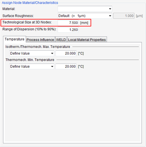
The technological size in FEMFAT considers the material endurance stress limit which decreases with increasing component dimensions. The imported shell thickness, which is averaged at the nodes in FEMFAT, is used as the technological size for FEM shell entities. For FEM solid entities, on the other hand, the user must explicitly specify the technological size as a numerical value in [mm] in the node properties. You can activate the technological sice influence factor in the menu "Influence Factor".
The sample thickness is also included in the analysis, where it should be noted that the sample thickness at five points is included in the material data, i.e. in the strength data for tension, compression, bending and shear, and again in the general S/N data. However, only the value from the general S/N data is used in the technological size influence!
Details from the FKM guideline
With the size influence activated in FEMFAT, an influence factor on the material alternating stress limit is calculated, in accordance with the FKM guideline [1, 2]. The "effective diameter" used in the equations there is identical to the "Technological size at 3D nodes" entered in FEMFAT for the node properties of the component.
In the following figure the influence of the technological size on the endurance stress limit is shown for various material classes. The corresponding FEMFAT material classes are given in brackets.
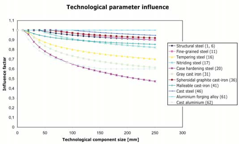
[1] FKM guideline "Numerical Strength Analyses for Machine Components in Steel, Cast Iron and Aluminum Materials", 4th Edition, 2002, www.vdma-verlag.de.
[2] FKM guideline "Analytical Strength Assessment", 5th Edition 2003, www.vdma-verlag.de.
Enabling the isothermal temperature influence means that the local operating temperature is taken into account at all analyzed nodes (usually upper temperature).
FEMFAT provides various analysis methods for this:
“FKM guideline” method
The isothermal temperature only affects the dynamic strength values in the Haigh diagram (vertical scaling).
“FEMFAT 4.5” method
This option changes both the dynamic strength parameters in the Haigh diagram (similar to the FKM guideline) and the static strength parameters (horizontal scaling of the Haigh diagram). The same formulae from the FKM guideline are used for modifying the yield stress and ultimate tensile stress. The user is warned if the temperature exceeds the range defined in the FKM guideline, and the influence factor is extrapolated on the basis of the implemented formulae.
“User defined” method
In this method, the temperature dependent material data specified by the user is taken into account; this data can be defined in the menu “Material data -> Properties at higher temperatures”. The temperature dependent fully reversed endurance limit and the ultimate tensile strength must be defined as a minimum for this method.
“FEMFAT 4.6” method (default)
This option is based on method 4.5, but in addition the cyclic coefficient of hardening K’ of the cyclic stress-strain curve is reduced in a similar way as the ultimate tensile strength. This means that the isothermal temperature influence is also correctly taken into account in the mean stress rearrangement of linear elastic stresses according to Neuber (FEMFAT plast module).
Isothermal temperature influence on Rm, Re and K´

One can see from the curves that all temperature influences based on FKM produce conservative results.
If you are unable to find the required material in the material database, you can also generate the data for the calculation on a few familiar properties of the material. The user has 2 options.
The first is called the 'stress-controlled' method by FEMFAT. Here you only need to specify the material class (Fig. 1) and the ultimate tensile strength for the material. Based on the predefined ratios taken from the FKM guideline, the system will now automatically generate all the missing material characteristics needed for the calculation (Fig. 2).
To increase the reliability of our conclusions, it would naturally be better if one was able to also pre-define the ultimate yield stress, pulsating load strength and ultimate compressive strength/alternating stress limit from specimen test data. However, one should be careful when changing materials outside of the material generator since the FEMFAT calculation uses a number of different relations based on the material data, for example the 'k' factor used to measure the ductility of the material.
The second method for generating a material is called the 'strain-controlled' method. The user not only needs to enter the material class (as in fig. 1), but also the data for ultimate tensile strength, yield stress and E/N curve (unnotched, polished samples, fully reversed tension/ compression) (fig. 3).
Finally, the number of cycles at the fatigue limit is also needed. Next, for this number of cycles, the strain amplitude is converted into a stress amplitude (corresponding to the fully reversed endurance limit). The fatigue strength exponent b is used to determine the gradient of the stress S/N curve (k=-1/b). After the material characteristics have been determined, you should then check the following and change where necessary: Survival probability, specimen diameter, elongation of rupture, check Haigh diagram & S/N curve for plausibility.
Since FEMFAT version 5.0 it is also possible to estimate parameters of materials with pores inside. In many cases as e.g. in Aluminum die cast components, there are areas with pores and defects, whereas surface layers are pore free. In FEMFAT a boundary layer model is provided for correct fatigue assessment of such cast components. Nevertheless the necessary parameters for material with and without pores are often not known. A new dialog for defect definition is now provided (fig. 4). Based on a pore free material or a material, where the maximum defect size is known (which is relevant for fatigue failure), material parameters can be derived for any other defect sizes.

Figure 1

Figure 2

Figure 3
Figure 4
FEMFAT provides an option for defining temperature- dependent material parameters (static and dynamic) and thus to take them into consideration in the fatigue analysis. The simplest solution is to import an existing material from the FEMFAT material database, e.g. the cast metal AlSi12CuNiMg.
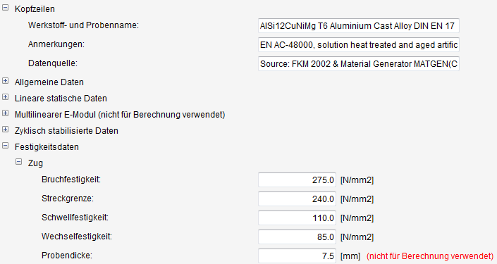
Right at the bottom of the "Material data" dialog there is an entry titled "Properties at high temperature". Here, value pairs consisting of the temperature and the corresponding material parameter can be entered.
Attention should be paid that the strength parameters correspond to the imported basic parameters at 20°C. For a user-defined assessment of the temperature influence at least the temperature-dependency of the ultimate tensile strength and the alternating stress limit must be given.
The remaining temperature-dependent material parameters can be estimated automatically by FEMFAT – although it is better to provide more temperature-dependent material properties, such as the pulsating stress limit, for example. This extended material can now be saved to the material database once again using the "Write to materials database" command and be used for subsequent analyses. It is adopted automatically for the current FEMFAT session. A nodal temperature distribution must now be defined as an "isothermal influence". Do not forget to activate the isothermal temperature influence in "Influence factors" and to change the method used to "user-defined".
Here, a simple example will be used to reveal the applicability of the FEMFAT plast method.
The same cyclic-plastic material data are used in FEMFAT and ABAQUS (parameters K´ and n´). The following analyses were performed on a fine-grain steel:
- ABAQUS with a cyclic-plastic material curve and true stress-strain definition with non-linear geometry.
- ABAQUS with linear material behavior and stress rearrangement using FEMFAT plast.
A notched, tensile specimen of steel with notch radius 0.7 mm, (d = 2.15) was analyzed for an alternating load of up to 40 kN (stress ratio R = -1). In Fig. 1 the stress history at the base of the notch can be seen for the Mises and max. principal normal stress. Initial plastification in the notch occurs at approx. 8 kN.
The Neuber rule applies to regions with limited local plastic zones. The individual regions are shown in Fig. 1. In region 1 (0-10 kN) local plastification restricted to the notch prevails.
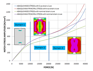
Fig. 1: Notch stress development in the notch base with plastic material behavior in ABAQUS
In region 2 (10-20 kN) the entire cross-section begins to plastify. In region 3 (above 20 kN) the entire cross-section plastifies. In our case the Neuber rule can be applied up to around 20 kN, because the initial cross-section plasticizes only very little up to this limit. Due to the loss of stiffness there is a large increase in local stresses at a load of 40 kN.
Fig. 2 shows a comparison of the stress amplitudes between ABAQUS and FEMFAT plast. The principal normal stress is used for redistribution in BASIC. The plastic analysis in ABAQUS uses the Mises equivalent stress for this purpose. This results in stress deviations in FEMFAT, but also because the node-averaged stresses are used for stress rearrangementin FEMFAT and not those at the element integration point.
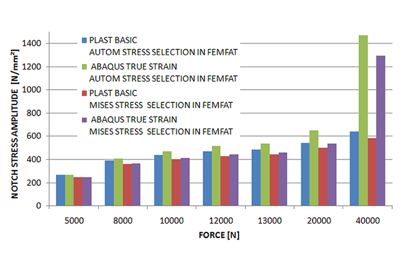
Fig. 2: Comparison of stress amplitudes from FEMFAT PLAST/ABAQUS
Summary:
Although a multi-axial stress state already exists in the notch, PLAST provides useful results up to approximately 15 kN (~ 0.3% plastic strain) for the local stress in the notch. If greater strains or stress multiaxiality are anticipated deviations may increase and a non-linear material law should then generally be employed.
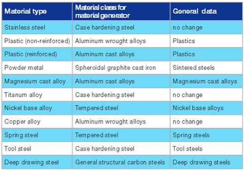
In the most simple case, a new data set is created with the material generator in FEMFAT by specifying the material class and at least the ultimate tensile strength. Sometimes, however, even the first step in this simple situation proves to be impossible: this happens when the desired material class (such as powder metal) is not available. For such cases you will find a table which shows the equivalent material classes we recommend.
After generating the material, the actual material class must still be specified in the general data (if available; see the 3rd column in the table).
Material properties must already be specified in the finite element simulation: Elements typically have a Physical Property (PID), which in turn refers to a Material Number (MID).
In FEMFAT, in addition to structure and stress results, material data and their assignment are an essential part of a durability analysis.
As of FEMFAT 5.4.3, the MID or PID from the imported FE structure can now be linked to FEMFAT material files (*.ffd) via a control file (*.fma) and an automatic assignment can be made. Thereby two steps (material import & assignment) can be saved in FEMFAT.
The structure of the fma file is a simple correspondence table: the first two columns include MID and PID, respectively, and the third column includes the FEMFAT material files. Columns 4 and 5 are optional input for material description as well as comments.
The corresponding FEMFAT materials are now assigned to the nodes according to their MID or PID. If both MID and PID are specified, the assignment is made for their intersection. If no MID or PID is specified, the ffd file listed is simply imported without further assignment.
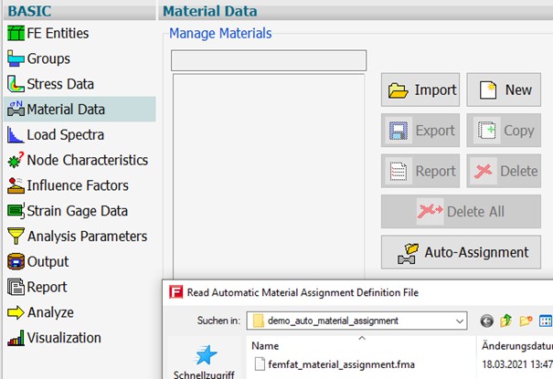
A complete example can be found in the directory <FEMFATInstallDir>\examples\demo_auto_material_assignment .
The example file femfat_material_assignment.fma (fma=femfat material automatism) is read in the menu "Material data" via the new button "Auto-Assignment".
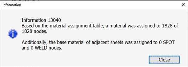
The displayed information confirms that a material has been assigned to all nodes in this case:
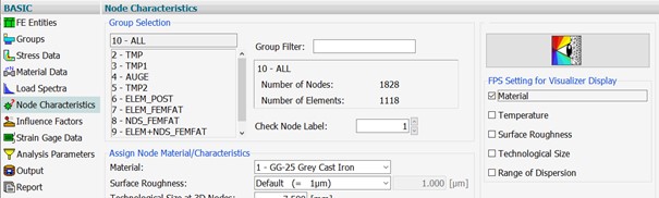
The material assignment can be checked particularly conveniently in the FEMFAT visualizer. To do this, activate the "Material" option in the "FPS Setting for VISUALIZER Display" in the "Node Characteristics" menu.
Currently, structural data in the format NASTRAN op2/bdf, MEDINA, I-DEAS MS-Universal, ANSYS cdb are supported. The possible number of readable materials is 500.
Cyclic stress-strain curves describe how materials behave under repeated (cyclic) loading.
This concept is different from the monotonous stress-strain curve obtained from a tensile test because the material's behavior changes under cyclic loading: cyclically softening materials have a stress-strain curve below the monotonous stress-strain curve, while cyclically hardening materials have a stress-strain curve above it. With increasing number of load cycles these effects fade and the material behavior stabilizes.
The stabilized cyclic stress-strain curves are crucial in FEMFAT plast for the Neuber stress re-arrangement to estimate local stresses in notched components.
Mathematically the cyclic stabilized stress-strain curves can be described in terms of the cyclic coefficient of hardening K´ and the cyclic exponent of hardening n’:
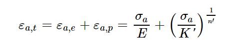
If K´ and/or n´ have not been defined by the user, they will be automatically generated by FEMFAT based on the Uniform Material Law (UML) [1], as a function of the material group and the ultimate tensile strength Rm.
Remark: The Uniform Material Law was developed based on specimen tests for specific material classes to generate a correlation based on the material class and the UTS of the material.
[1] Bäumel, A. jr.; Seeger, T.: Materials data for cyclic loading, Supplement 1. Elsevier,
Amsterdam (1990).
In the Check Input Data file (*.cid) that can be created by FEMFAT, the stress representation depends on the selected module:
- In BASIC module, one of the principal normal stresses is output.
- For amplitude stress:
stress = max [|σ1|, |σ2|, |σ3|] - For mean stress, the maximum absolute principal stress is used, but with the sign of the largest absolute value |σk|=max [|σ1, |σ2|, |σ3|]
stress = sgn(σk) * max [|σ1|, |σ2|, |σ3|]
- For amplitude stress:
- In MAX module, the Mises stress is used, multiplied by the channel factor and the maximum absolute value of the time history of each channel.
FEMFAT break is a very practical tool for computing static safety factors from linear-elastic FEM stresses. For abrupt, infrequent loads (e.g. transmission jump starting, chassis-verge stone contact) it is recommended to perform a FEMFAT break analysis prior to the fatigue analysis. If an insufficient static safety factor results here (safety factor smaller than 1.0) the component is statically underdesigned.
The static safety factor is used to evaluate the local elongation capacity of the material until cracking under a monotonic load.
Please note that FEMFAT break cannot assess the global failure (fracturing, breakage) of a component (unless the material is highly brittle), but only the local material failure due to insufficient ductility. This means that initial damage (small crack) may be caused by high load peaks, which leads to further crack growth under subsequent operating loads, and finally to failure. In addition, it is assumed that the constant load is not applied highly dynamically; i.e. BREAK does not take strain rate effects into consideration. Influences in the BREAK module the notch influence is taken into consideration by means of the relative stress gradient. Required material parameters:
- Young’s modulus
- Static tensile strength Rm
- Static compressive strength
- Static shear strength
- Static elongation at rupture A5
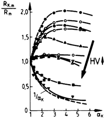
Image: Ratio of notch tensile strength to tensile strength as a function of the stress concentration factor and Vickers hardness, as a measure for ductility.
The ratio of bending to tensile strength defines the impact of the gradient influence; i.e. the greater the ratio, the greater the strengthening and the smaller the (negative) notch influence on the static component strength. Under static loads, the notch influence may even reverse, in contrast to cyclic loads. That is, it may have a positive influence on component strength as a function of the ductility of the material, see diagram (source: Systematische Beurteilung technischer Schadensfälle, third revised/extended edition, G. Lange, Informationsgesellschaft Verlag). The cause of this is that a ductile material only begins to yield under higher loads due to the multi-axial stress state in the notch. Brittle failure dominates in a brittle material.
Evaluation Method
By default the maximum principal stress is adopted as the relevant value for gray cast iron and a modified Mises stress taking the shear strength into consideration for all other materials. The ultimate tensile or compressive strength is adopted for gray cast iron, as a function of the prevalent principal normal stress components. Effective failure strength is computed for ductile materials by interpolation. The static elongation of rupture is very important in BREAK, because it is used to compute the maximum local notch strength. That is, the static safety factor in sharp notches increases in direct proportion to the static elongation. In addition, it should be noted that the static elongation in the component may drop locally, in particular in light metals and for poor casting processes.
Since FEMFAT version 5.0 BREAK is also available in MAX. There at each node a separate static safety assessment is performed for each time point. At the currently analyzed node the time point with minimum static safety factor is assumed to be critical and the corresponding results are written into the dma- and pro-file.
FEMFAT basic provides the possibility of reading a third load case, designated as constant stress (σc), at the given amplitude and mean stress (σa, σm). These could arise from internal stresses or screw preloadings. When the constant stress effect (influence factors -> general factors; Fig. 1) is activated, the constant stress is included in the mean stress during the calculation. The difference with regard to the mean stress data set is in the definition of the load spectra, where only the mean stress is scaled with the “mean stress factor” (F_M) for each step. In the case of the fatigue strength analysis, the constant tensile stress with the R = const. option (one of the FKM overload situations) is taken into account as a shift to the right in the Haigh diagram (Fig. 2).
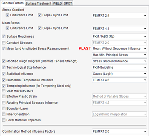
Figure 1
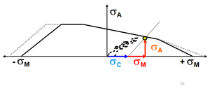
Figure 2
Besides the material, component geometry and stress conditions, the manufacturing process has a major influence on the fatigue behavior of a component.
In FEMFAT the following surface treatments are available:
- Shot peening (acc. to FKM, Eurocode or BS),
- Rolling (to FKM),
- Carburizing (to FKM),
- Nitriding (to FKM),
Here, the condition prior to nitriding can also be taken into consideration: Tempered or normalized
- Inductive hardening (to FKM),
- Flame hardening (to FKM).
"Node properties menu" for the current group
For these treatments it is important that the Technological size at 3D nodes is given in "Node properties" (see image). This technological size is automatically determined from the mean shell thicknesses for shell structures. For example, the technological size is the wall thickness of a tube or the diameter of a shaft at the point where the surface treatment is carried out. Other influences, such as the relative stress gradient and the material strength are automatically taken into consideration by FEMFAT.
The Surface treatment factor provides a good option for incorporating experiences from testing into analysis. This directly alters the local endurance stress limit.
One common technological influence is the Surface roughness, which can be assigned to the current group. The S/N curves of the material data are generally defined for a smooth, un-notched specimen for alternating tensile-compressive loading. This means that a change in the surface roughness also changes the endurance stress limit, the slope and the endurance cycle limit of the local S/N curve at the node, including as a function of the material itself. In the methods listed under "Influence factors" one can also select between mean roughness depth Rz (to TGL or FKM) or the maximum roughness depth Rt (IABG) of the assessed component surface. The former TGL Standard - replaced by the FKM Guideline in 1994 - is no longer recommended.
FEMFAT also includes an option for taking the Tempering condition into consideration for tempered steels. If the tempering condition changes (= new ultimate tensile strength) all governing material parameters are adapted to the new tempering condition. Following this, do not forget to activate the process influences in "Influence factors" (surface roughness, technological parameter influence, tempering influence...)!
Often, after an endurance safety analysis has been made, the additional question arises of how many cycles the component can sustain under the load which is to be applied. In the case of single-level load spectra, this question can be answered by means of a simple conversion between safety factor and fatigue life:
If the safety factor is less than 1, in order to calculate the sustainable number of cycles N, the degree of utilization (= reciprocal of the safety factor 1/SFA) is raised to the power of the negative slope k of the (local) S/N curve and multiplied by the (local) endurance cycle limit ND:
N =ND* (1/SFA ) -k
If the safety factor is greater than 1, the conversion depends on the Miner rule used:
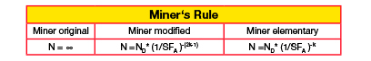
By the way, this conversion can be carried out very conveniently using the FEMFAT Results Manager in which the above-mentioned case differentiation for the safety factor can be made automatically with the help of the formula Editor.
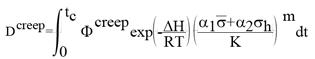
In HEAT the total damage for thermomechanical fatigue consists of three terms:
Dmech ... the mechanical damage component according to COFFIN/MANSON
Dox ....... the oxidation damage/ambient damage component
Dcreep ... the creep damage component
Dtotal = Dmech + Dox + Dcreep
In the oxidation damage according to BOISMIER, KADIOGLU and SEHITOGLU the oxidation phase Fox and the strain rate (e) are very highly dependent on the strain history over time.
Creep damage is most prominent for an in-phase TMF load (mechanical loads enhance thermal strain) and is integrated over the cycle time. This naturally implies that damage is time-dependent.
The time information (unit: seconds) can be defined in a number of ways. Either the step time from the stress, strain or temperature results can be used (which makes more uncommon step time definitions necessary) or a separate table is imported as a text file. This can be performed on the "Time information" tab.
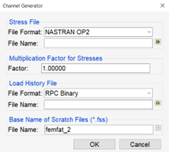
In ChannelMAX, you can automatically assign the load time histories of a load history file to the stress data of a stress file. This process is streamlined through the Channel Generator, which can be accessed from the Channels menu by clicking the corresponding icon.
How It Works
The automatic channel definition functions by linking the stress data to a load time series through a unique string. This string is verified for equality and must be defined according to the specific interface. The number of channels generated is determined by the number of matches found. Specifically, this means that the label in the subcase definition (for the NASTRAN interface) or the name in the step/load case definition (for the ABAQUS interface) must correspond to the channel name in the load history file.
Supported Interfaces
The Channel Generator supports the following interfaces:
- Stress Files: Nastran op2 and Abaqus odb
- Load History Data: RPC ASCII and binary
By utilizing these supported interfaces, ChannelMAX ensures that the process of matching load time histories to stress data is both efficient and accurate.
Steps to Use the Channel Generator
- Open ChannelMAX: Import the structure file.
- Navigate to the Channels menu.
- Start the Channel Generator: Click on the icon “Generator” to initiate the process.
- Specify the Stress file and Load History file: Ensure that the unique strings for the stress data and load time series are defined according to the respective interface.
- Generate Channels: The Channel Generator will automatically create channels based on the number of matches found.
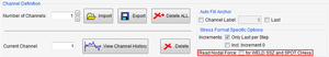
It is possible to simulate the repetition of the load sequence in TransMAX by definition of “Number of Calculation Sequences” greater than 1. If a factor of 100 is given for 10 time points, it corresponds to a total number of 1,000 time points. The increase in this factor is useful for damage calculations, in order to reduce the effect of the Rainflow residuum on the result (not necessary for the Default Rainflow Counting Method).
Caution: When calculating the endurance safety factor, the factor does not affect the result and should remain unchanged (default value 1)!
This repetition factor can be changed as required without necessity to recreate the scratch files, because the duplication of the time points only takes place during the calculation.
As the number of time points is directly corresponding to the calculation time, the repetition should be selected with caution, e.g. in the 10-100 (see figure).
In order to save considerable computation time it is possible to compress the load-time histories imported into ChannelMAX. After pressing the "Compress load-time history" button intermediate points that generally exercise no influence on the Rainflow counting can be filtered out on the one hand ("peak slicing"); on the other hand, cycles with small amplitudes can be ignored ("cycle omission"). Three different options are available for defining the threshold value of these partial cycles, whereby one of the options takes the component stresses into consideration (see figure 1 below).
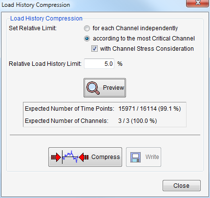
Figure1
The largest occurring stress for the entire loading history of the current analysis group is adopted for filtering. In conjunction with the user-defined filter limit (default 5%) this results in a stress that filters the small cycles of all loading channels.
This leads to a number of advantages:
- Stress directions to which the structure's reaction is highly unresponsive (cf. beam under tension/bending) are heavily filtered.
- Unit differences between loading channels are no longer important (e.g. channels defined in [kN] are not filtered preferentially to channels in [N]).
- Various load types such as force, moment, pressure, etc., are correctly evaluated and compressed in relation to one another.
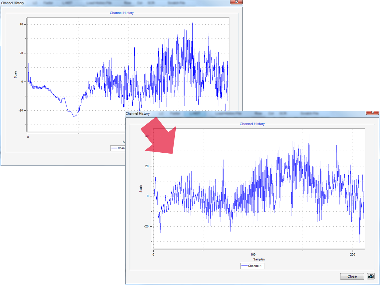
Figure 2: 1000 samples (original load list), 211 samples (compressed list)
This method is especially efficient if only small areas of the structure are to be analyzed: because many stress directions often only cause very minor stresses at the respective location, these channels can be highly compressed or even deleted, resulting in a substantial reduction in computation time. The import of the load-time histories and the compression are both very fast. This procedure can therefore be easily repeated (for several critical locations).
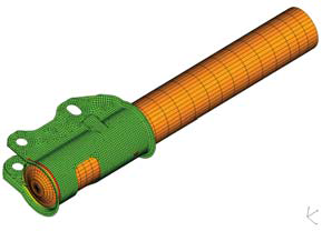
ChannelMAX also enables users to carry out fatigue analyses on non-linear results from calculations- e.g. due to contact problems. Such nonlinearities must be handled differently in ChannelMAX, in contrast to TransMAX where they are already taken into account when calculating the stress sequence. A good example here would be a wheel mount for which a contact condition applies between the green and orange-coloured component. A lateral force is introduced as a load at the upper end of the wheel mount. It is not simply a question of combining the non-linear stress results with the stress history shown below (in black), which contains both positive and negative values. Doing so would completely misrepresent the contact relationships.
In order to continue being able to perform a FEMFAT ChanneIMAX calculation, the following two steps are required:
1. The stress history is divided into a positive component and a negative component:
Original signal:
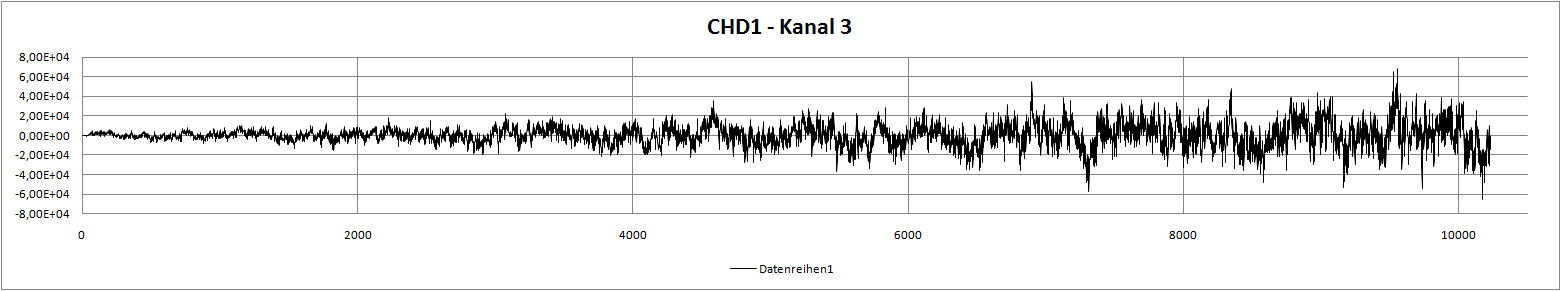
Positive component:
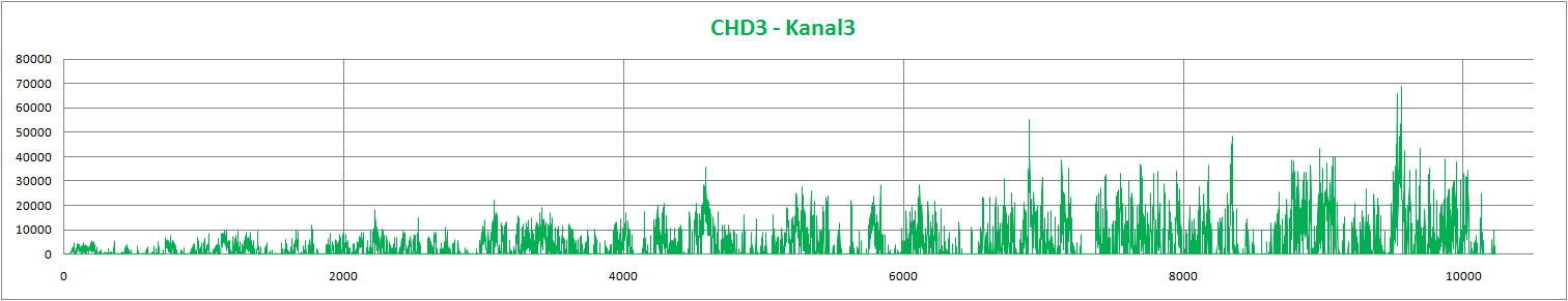
Negative component:
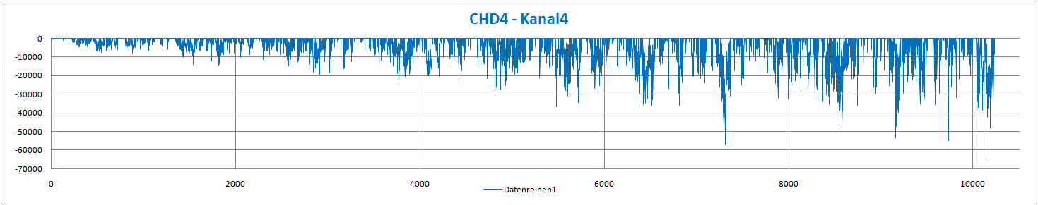
2. In addition, characteristic working points (=load levels) need to be identified from the load history with damage-relevant contents. This must be done for the positive and negative area. In this example, this part is approx. 75% of the maximum loading, i.e. approx. 700N for the positive and 400N for the negative component. These two characteristic loads are now used to perform the non-linear FE-analyses. The stress results obtained from this calculation are imported into FEMFAT as “new” unit load cases for the associated partitioned loading histories in ChannelMAX. It is important to ensure that the factor for the stress results is entered as 1/700 for the first channel and 1/400 for the second channel to achieve the correct stress level once again.

After the FEMFAT analysis, the user finally comes out with a damage distribution taking account as far as possible of non-linear contact effects. This method can also be used with multi-axial loads. However, in this case, contact states may appear less accurate due to the non-linear transfer effects of multiple channels. This effect is rare however since in most cases only a few directions of the applied force dominate at a particular moment. In any case, what matters is the correct working point, which is located close to the existing peaks in cases of practical relevance (the reason for this is simply because the largest peaks in load usually cause the highest partial damages).
You should be careful with initial pre-stresses: such stresses should be deducted from the operating load states and an additional constant channel defined.
In summary, what we have here is a practical method which offers sufficient accuracy in most cases, and which offers enormous time benefits (up to several orders of magnitude) compared over analyzing of many non-linear stress states together with a TransMAX analysis.
Simple load signals (constant Signal, cosine or triangle signal) can be definied directly in ChannelMAX.
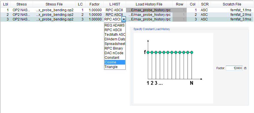
An extension of the channel definition for simple generation of signals was created (as a supplement to the diverse interfaces).
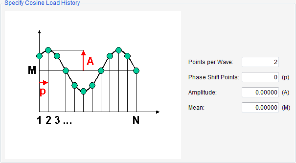
The cosine and triangle Signal allow specifying the number of sampling points per wave, the amplitude, the mean leveland a phase shift. The total number of samples is not queried until the load histories are scratched, if no load data are imported from interfaces. Typical applications for constant signals include bolt pre-stresses. Cosine signals can be used for rotating loads for example (2 load channels with 90% phase displacement).
In some loading situations, e.g. in crankshafts subject to combined bending/torsional loads, a local change or rotation in the directions of the principal stresses may occur with time.
Tests using combined bending/torsional alternating loads and 90 degree phase shift have shown that for ductile materials (tempered steel) the critical cutting plane method overestimates the lifetime (e.g. see FKM report "Multiaxial Fatigue Analysis, 2002"). In FEMFAT MAX it is possible to correlate the lifetime using "Influence of rotating principal stresses".
The local S/N curve is reduced as a function of a statistical degree of multiaxiality lying between 0 (= proportional load with constant direction of principal stresses) and 1 (= heavily nonproportional load with directions of principal stresses changeable with time).
The influence thus results in a reduction in lifetime in ductile materials.
No impact is defined for brittle cast materials (gray cast iron, cast Al, cast Mg).
We recommend activating the influence of rotating principal stresses. However, in certain cases, e.g. where high constant stresses are involved (bolt pre-stresses, residual stresses), the results may be conservative.
In some loading situations, e.g. in crankshafts subject to combined bending/torsional loads, a local change or rotation in the directions of the principal stresses may occur with time. Tests using combined bending/torsional alternating loads and 90 degree phase shift have shown that for ductile materials (tempered steel) the critical cutting plane method overestimates the lifetime (e.g. see FKM report "Multiaxial Fatigue Analysis, 2002"). In FEMFAT MAX it is possible to correlate the lifetime using "Influence of rotating principal stresses". The local S/N curve is reduced as a function of a statistical degree of multiaxiality lying between 0 (= proportional load with constant direction of principal stresses) and 1 (= heavily nonproportional load with directions of principal stresses changeable with time). The influence thus results in a reduction in lifetime in ductile materials. No impact is defined for brittle cast materials (gray cast iron, cast Al, cast Mg).
We recommend activating the influence of rotating principal stresses. However, in certain cases, e.g. where high constant stresses are involved (bolt pre-stresses, residual stresses), the results may be conservative.
Option 2 – Compress load history
One procedure for eliminating less relevant channels is the loadtime data reduction provided by ChannelMAX. To do this, the settings “for the most critical channel” and “with consideration of channel stress” must be selected in the compression menu (see Fig. 2 top). The advantage here is that channels with small stress portions are completely deleted. In addition, data points between the minimum and the maximum are eliminated, as well as small amplitudes below a user-defined limit which only cause a minor damage share (Fig. 2 bottom). Beside the advantage of taking phase shifts into account, a considerable reduction in computation time results.
Option 3 - VISUALIZER
The FEMFAT VISUALIZER provides an option for also visualizing the corresponding load factors multiplied by the stresses from the unit load case for individual nodes (from the “Detailed Result Group”), in addition to the equivalent stress history, damage history and partial damages. After clicking any point in time with a large damage increase, for example, a diagram containing the corresponding stress values per channel is displayed. They are sorted according to size for clarity. From this, in turn, it is possible to derive which load channels contain a high damage component.
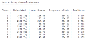
Figure 1: Max arising channel-stresses
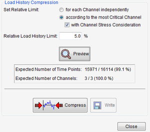
Figure 2: Load history compression
The default settings regarding influence factors and analysis parameters reflect our recommendations for the fatigue analysis. To follow your own “guidelines” in the department or in the group, you sometimes have to overwrite these defaults.
We provided the first help with the templates in FEMFAT 5.1 (2014). They can be found in the FEMFAT installation directory / templates and include the weld sensitivity analysis, the recommended settings for GL 2010 and the evaluation of elastomers.
Calling and reading job files is easy with the icon on the graphical user interface , but as such is not recorded in the ffj file. Instead, the read lines are appended to the current job file.
In the batch job such a call has to be inserted with the TCL / TK command "source" (the absolut path must be specified or a variable previously defined in the program must be used, as here "installation_path"):
source $installation_path/templates/WELD_Sensitivity_Damage_gap.ffj
The previously described use of variables with the "set" command to assign the "installation_path" the standard installation directory of FEMFAT 5.4 then looks like this:
set installation_path „C:/Program Files/ECS/FEMFAT5.4“
If a job in which another job was read is saved after this action, it is no longer the call of the template or the job that is saved, but the lines from the template! So you have to decide whether you want to keep / save the calculated job files or the previously prepared job file or both.
Other TCL / TK commands that make it easier for you to design your jobs with FEMFAT can also be found in the templates for the WELD sensitivity analysis.
However, we would like to point out again that manually edited job files are not the standard and can only be examined by our support with additional effort.
When evaluating rotating components in FEMFAT, it is crucial to understand how element nodal stresses are transformed and output. The stress data at the nodes must be passed to FEMFAT in the form of stress tensors. It is assumed that the stress data are available as element nodal stresses, i.e., node-related for the individual elements, and defined in the global Cartesian coordinate system. This is necessary for correct stress averaging. Shell stresses are often, but not always, present in a local element coordinate system, depending on the solver and solver settings. Local element coordinate systems can also be defined differently depending on the solver.
For Ansys interface in FEMFAT, the transformation of element nodal stresses into the global coordinate system is performed for shell elements of types 43, 63, 93, 181, 190, and 281. For these elements, the element nodal stresses in the *.rst file are available in the rotating element coordinate system.
For solid elements, there are usually solver-specific options/settings to output stresses in the local coordinate system. In ABAQUS, for example, a material coordinate system can be generated (in combination with "Ignore inconsistent transformation data" in FEMFAT).
In Ansys Mechanical, you can output stresses globally or in the rotating element coordinate system during postprocessing, provided large deformations are activated and you select the Solution Coordinate System. This option is also available in MAPDL.
With 'large deformations' active in Ansys, solid stresses are correctly imported into FEMFAT in the rotating element coordinate system. The stress components in Ansys Mechanical for rotated solid elements will differ between the global and solution coordinate systems, and the FEMFAT visualizer will match the solution coordinate system's stress components.
If the nodal forces are to be imported for a FEMFAT spot (JSAE method) or FEMFAT weld(SSZ/MSZ method) analysis, the corresponding check box (see figure) must first be activated. This option prevents excessive memory use. Note: Node forces can currently be imported from NASTRAN op2, Abaqus otb and MEDINA bof.
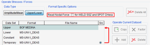
GUI for the node forces in BASIC
GUI for the node forces in MAX
Generally speaking, FEMFAT spot gives you the option of using the available stress concept (nugget elements) or force concept (connectors) either separately or combined.
However, it should be mentioned that the stress concept should not be combined with the force concept within a single flange. The reason for this is that the stiffness varies between the two concepts. Joints such as those with CWELD elements (force concept) are normally stiffer than FEMFAT element nuggets (stress concept). If a nugget is modeled next to a CWELD, this will result in the CWELD joint taking up more of the load flow, resulting in increased damage. The damage of the nugget will thereby decrease. Because of this, the same type of joint should be used within large areas (entire flange length, vehicle area) if you want to combine the two concepts
FEMFAT has its own calculation concept for the assessment of joints. Therefore it is necessary to do a remeshing of the basic structure.
Following procedure is very helpful for the remeshing, in case the spot-diameter is chosen according to the sheet thickness or the diameter matrix in the spot database.
Step 1: Definition of the center nodes and connecting elements. When there are failures it is very easy to correct them. Possible reasons may be double definition of CDHs.
Step 2: FEMFAT spot remeshing with mesh refinement.
Please note that after the remeshing the stress analysis has to be done once again.
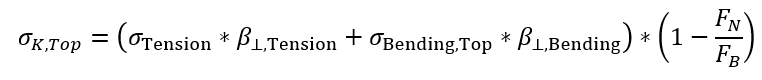
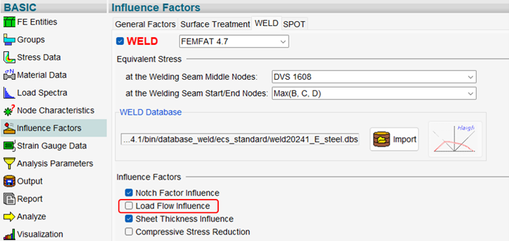
For combined WELD nodes with node attributes C103, C104, C105, C108, C109, the power flow over neighboring elements is not considered. This means that only the first part of the notch stress formula is used, notch factor 3 is excluded from the calculation:
Please note: deactivating the Load Flow influence on the GUI has a different effect.
In this case, the simplified formula is used:
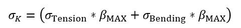
Where
is the maximum notch factor from the WELD database.
In FEMFAT weld, all sheets of a seam are evaluated with the same assessment distance when automatic stress correction is active. The option “Use Assessment Distance Zero for Root” overrules this convention for sheets that only have root notch factors on one sheet side (no weld toe). An example is the one-sided T-joint and the element with material 201 or 202 resp., see figure 1.
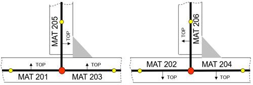
Figure 1: Modelling Guideline excerpt for T-weld with one-sides fillet weld
Specifically for single-sided weld joints on the side opposite the seam, the assessment distance would move even further away from the root with the default settings.
The option “Use Assessment Distance Zero for Root” avoids this and the evaluation takes places directly at the weld. Sheet sides with weld toes continue to be evaluated at the specified assessment distance.
In order to check and validate weld node analysis results, any possible source of errors are written as WARNING messages to the message file during automatic stress correction.
WARNING messages may occur. They only point out to the user that unusual conditions occur at the weld element or weld node in question, but need not be a direct cause of a false result.
WARNINGS during weld environment examination:
| Error no. | Description |
|---|---|
| W11461 | All element nodes are declared as weld nodes at the shell element in question. This indicates to the program that welds are analyzed at all element edges of this element. This does not correspond to the requirements of the modeling guidelines. This can lead to an interpretation error, in that additional welds are considered at weld edges that are not intended as such in the structure. The damage result or the endurance stress limit safety factor at the nodes in question may for this reason be too conservative for certain stress conditions. |
| W11462 | Although the weld node in question was declared as simple weld node (C100-C102, C106 or C107), it possesses differing joint types or weld types. The load flow across the neighboring element given in the weld database can therefore not be taken into consideration. Where simple welds are involved, the program checks that all neighboring weld elements belong to one joint type and weld type. Only in this case is it possible to consider the load flow across neighboring elements. WARNING 11462 can be subdued by declaring, where necessary, weld nodes as combined weld nodes (C103-C105, C108 or C109). |
| W11463 | At least one element, which was not declared as a weld element, is connected to the simple weld node in question. That is, the material property label of this element is not between 100 and 499. In principal, it is possible to attach elements other than weld elements to a weld node. However, the stresses in these elements are ignored during the weld assessment. WARNING 11463 can be subdued by declaring weld nodes as combined weld nodes (C103, C104, or C105). |
| W11464 | More than one defined neighboring element was found for the node in question. The load flow across the neighboring element can therefore not be considered. |
Table 1: WARNING messages during weld environment examination
ERROR messages on the other hand indicate false results or a false interpretation at the weld node concerned.
These occur because of gross breaches of the regulations of the weld modeling guidelines and can generally be rapidly remedied in the preprocessor without renewed FEM stress analysis. They are intended to point out to the user that conditions occur at the weld node in question that are fundamentally erroneous. Erroneous weld nodes are subsequently treated and assessed as normal base material nodes. Analysis of further, correct nodes is not influenced by this.
ERRORS during weld environment examination => weld nodes are treated as base material node.
| Error no. | Description |
|---|---|
| E11451 | There is no assessable element at the weld node in question. The node therefore cannot be evaluated as a weld by FEMFAT. This is generally due to an error in coloring of the weld nodes in the FEM preprocessor. Because the node is not connected to a shell element assessable as a weld, it is of no further meaning for the FEMFAT weld evaluation. |
| E11452 | No neighboring weld element was found for the weld node in question. The node is subsequently treated as a base material node. This indicates a modeling error in terms of the weld modeling guidelines. A minimum of one weld element must be connected to a weld node. |
| E11453 | No neighboring weld element, connected via an element edge, was found for the weld node in question. The node is subsequently treated as a base material node. |
| E11454 | No neighboring weld node, connected via a weld element edge, was found for the weld node in question. Therefore, no spatial weld course can be calculated, as the weld has a length of 0.The node is subsequently treated as a base material node. |
Table 2: Error messages during weld environment examination
Warning messages in the message file due to automatic stress correction
If, under certain circumstances, such WARNING messages occur it means that the "Automatic stress correction" (if activated) could not act at the node label in question. The corresponding weld node is then assessed without automatic stress correction, i.e. the element stress tensor of the current weld element is used. Such a WARNING message has no effect on the subsequent analysis of the remaining weld nodes.
Error in automatic stress correction => weld node is analysed without stress correction.
| Error no. | Designation | Description |
|---|---|---|
| W11431 | Weld modeling error | Either all nodes of a quadrilateral shell element were defined as weld nodes or an element with a weld material label possesses no weld nodes. |
| W11432 | No stress result for the element | The weld or neighboring element has no stresses. |
| W11433 | No neighboring element | No neighboring element was found when searching for the assessment point, e.g. if the assessment point lies outside the entity. |
| W11434 | Neighboring element not the required element type | The neighboring element must be a linear or parabolic shell element. |
| W11435 | Varying element thicknesses | The thicknesses of the neighboring and the weld element differ. |
| W11436 | Geometry not suitable for stress correction | When stress correction is performed for a coarse FEM mesh, the stress at the assessment point is found by linear interpolation between weld element and neighboring element. For this interpolation to provide correct results, the geometry of the FE-mesh will be checked:
|
| W11437 | The weld FEM mesh is too fine. | When stress correction is performed for a coarse FEM mesh, the stress at the assessment point is found by linear interpolation between weld element and neighboring element.
|
| W11438 | No nodes found near the assessment point belonging to the relevant neighboring element | If the distance from the weld seam of the center point of a neighboring element is greater than the distance of the assessment point, the node of the neighboring element with a minimum distance to the assessment point is used for weighted stress averaging. If this node with the smallest distance to the assessment point is not found, WARNING 11438 is written to the message file. |
Table 3: Error messages arising from automatic stress correction
Warning messages in the message file due to force-based assessment using the SSZ/MSZ method
If the SSZ or MSZ method was selected as the evaluation method, FEMFAT tries to determine the line loads based on the weld element node forces and to calculate structural stresses from them. If the line loads cannot be determined the element is automatically analyzed using the FEMFAT 4.7 default analysis method based on the FEM stresses. A WARNING message is then written to the message file (*.msg).
WARNING messages for the SSZ/MSZ method:
| No. | WARNING message | Description | Assessment method |
|---|---|---|---|
| W11401 | Error when determining the web plate angle ALFA. | The normal vector of the web or base plate could not be determined. The web plate angle is calculated based on the normal vector of the base and web plate element. These normal vectors are determined with the aid of a non-weld node of the relevant weld element. Such a node could not be found. A default value ALPHA = 45° or 90° is used. | SSZ/MSZ method |
| W11402 | Error when determining the web plate angle ALFA. | Too few input data for cosine calculation.COS(ALPHA) could not be determined from the Inproduct when calculating the web plate angle from the element normals. One normal vector is zero. A default value ALPHA = 45° or 90° is used. | SSZ/MSZ method |
| W11403 | Error when determining the web plate angle ALFA. | If the angle between the normal vectors of the base and web plates is smaller than 1.14° is, this WARNING message is given.A default value ALPHA = 45° or 90° is used. | SSZ/MSZ method |
| W11404 | Error when determining the web plate angle ALFA. | Relevant elements for calculating the angle were not found.Web plate and base plate are identified based on the MAT labels in accordance with the modeling guideline. The MAT labels must also be listed in the weld database for the SSZ entries (ZA, ZB or ZC identifier).A default value ALPHA = 45° or 90° is used. | SSZ/MSZ method |
| W11420 | at element withlabel ….. | If the web plate angle is too small (1.14°<ALPHA<15°), then the element is evaluated as a lap joint. | SSZ/MSZ method |
| W11421 | The sheet thicknesses at the SSZ joint could not be determined.The weld evaluation is stress-based (standard WELD method)! | Both sheet thicknesses at the joint could not be determined or are zero. Check that the modelling guideline was adhered to. | FEMFAT 4.7 |
| W11422 | Sheet thickness 1 at the SSZ joint could not be determined.Thickness 1 is set to thickness 2! | Sheet thickness of side 1 could not be determined or is zero. Check that the modelling guideline was adhered to. | SSZ/MSZ method |
| W11423 | Sheet thickness 2 at the SSZ joint could not be determined.Thickness 2 is set to thickness 1! | Sheet thickness of side 2 could not be determined or is zero. Check that the modelling guideline was adhered to. | SSZ/MSZ method |
| W11424 | SSZ geometry parameter outside of allowable range. | The geometry parameters are checked for plausibility. If the value is outside the permissible range (see Table 25), the default vale from the database is used | SSZ/MSZ method |
| W11425 | at element withlabel ….. | The MAT label of the element is not associated with a SSZ joint. The MAT labels associated with a SSZ joint are stored in the weld database with the ZA, ZB and ZC identifiers. If the MAT label is not entered there the element is not recognized as a SSZ joint and evaluation is stress-based. | FEMFAT 4.7 |
| W11426 | at element withlabel ….. | The forces at the nodes are all zero or very small. If all 6 components (3 forces, 3 moments) of the force vector are zero or are very small, evaluation is stress-based (default WELD method). | FEMFAT 4.7 |
| W11427 | at element withlabel ….. | The MAT label of the element is associated with a SSZ joint but allocation to a joint side failed. Check that the modelling guideline was adhered to. The element evaluation is stress-based. | FEMFAT 4.7 |
Table 4: WARNING messages for SSZ/MSZ method
For simple weld fatigue assessments, the stresses acting on the finite elements defining the weld are often used. In this case the evaluated stresses are largely a function of the element size. Figure 1 shows the distribution of the normal stress perpendicular to the weld for a lap joint with four different element sizes. It can be seen that the maximum stress is a function of the element size on the one hand, and that, on the other hand, the stresses are almost identical at a relatively small distance.
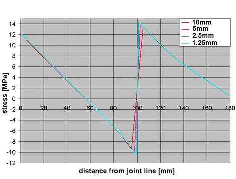
With the aid of the automatic stress correction in WELD the user can specify the assessment distance D from the weld where the stresses are identified, regardless of the element size. The minimum sheet thickness at the joint is used by default; i.e. the assessment point is near the weld transition zone. First, a neighboring element to the current weld element is searched for. If the center point of the neighboring element is at a greater distance than the assessment point, the stresses of the weld element and the neighboring element are interpolated.
If the center point of the neighboring element is at a lesser distance than the assessment point a search algorithm is started. The algorithm searches along an interpolation plane perpendicular to the weld for an element with an element center further from the weld than the assessment distance, and with the smallest distance from the interpolation plane.
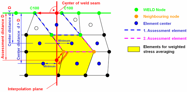
All elements attached to the node with the smallest distance to the assessment point are then used to acquire a weighted mean for the stress components:
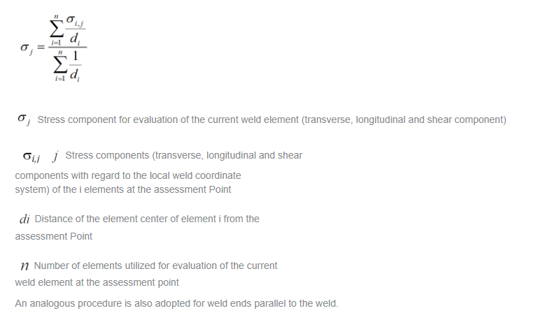
Because FEMFAT weld uses an ASCII format database for weld assessment it is also possible for the user to adapt the database to their requirements or to expand it if a special weld type is not supported. The database includes notch factors, weld S/N curves, weld Haigh diagrams, etc. During analysis FEMFAT differentiates between the shell membrane and bending stresses. This makes it necessary to enter notch factors for both types of loading when expanding the database. The notch factors are usually computed using a Radaj model (1 mm rounding radius for root/toe and 10 mm sheet thickness), which is subject to various membrane and bending load cases. The factors acquired are related to evaluations perpendicular to the weld direction. When evaluating Radaj models it should be noted that the stress component in the direction of loading is adopted (notch factor = notch stress/nominal stress).
The factors from a similar joint can be adopted for the weld end, or they can be determined by means of a 3D model (structure analogous to the Radaj model). Once the evaluated notch factors have been entered the equivalent element list must be appropriately expanded for joint types with neighboring elements (e.g. T-joint), see the example below:
$ Substitute element allocation
$ ------------------------------
$ T-joint, one-sided fillet weld with root undercut
$ ---------------------------------------------------------------
R 201 202
R 202 201
R 203 204
R 205 206
R 206 205
If the nodal forces based SSZ/MSZ method is used in addition to the standard FEMFAT method, the new MAT labels should also be entered in the SSZ parameter list. The SID labels must be adapted to make the newly defined welds available in VISUALIZER. Ensure that the predefined SID ranges are used (see FEMFAT weld manual). Now the small, detailed model displayed in VISUALIZER as a visual feedback must be entered in the database as a polygon and the image stored in *.gif format. This image must be added to the "weld_images" folder, which is located in turn in the WELD database folder.
The FEMFAT installation package includes the ECS standard (notch stress concept) as well as the WELD databases according to BS7608, DVS952 and Eurocode 3 & 9.
In addition to this, there are further databases available on request for standardcompliant weld analysis according to
- DVS1608 & DVS1612,
- IIW,
- FKM (nominal or notch-stress based).
Please keep in mind here that the databases offered contain a selection of FAT classes and/or joints.
If the desired FAT class is absent, we would be happy to assist you in enhancing the WELD database. Due to the fact that the S/N curves of the standards reference nominal stresses but FEMFAT processes structural stresses, the results will lie on the conservative side in many cases.
If the nodal forces are to be imported for a FEMFAT spot (JSAE method) or FEMFAT weld (SSZ/MSZ method) analysis, the corresponding check box (see figure) must first be activated. This option prevents excessive memory use. Note: Node forces can currently be imported from NASTRAN op2, Abaqus otb and MEDINA bof.
GUI for the node forces in BASIC
GUI for the node forces in MAX
For the output and display of results at weld nodes, there are three result positions available in the VISUALIZER:
Visualization of the analysis results as a middle or end node, Visualization of the results at the weld root or at the weld toe, Visualization of the results of the individual stress components (Normal stress perpendicular to and parallel to weld, Shear stress, Equivalent stress).
Basically, the critical values for each of the three categories are first displayed when invoking the results. The user-defined selection of the evaluation positions can be made via a drop-down menu.
However, it should be noted that all results for root & toe are not available for all involved sheets / elements at one weld seam node. Only those weld toes and roots are calculated for which notch factors have been defined in the WELD database. The values of the most critical element are then displayed according to the settings.
This means, for example, that if the critical element has no weld toe at all (because it lies on the side away from the seam like an element of type 202, pictured right), then the value is also not available. In VISUALIZER, when „Toe“ is selected for such a weld node, „Not Analysed“ is displayed, cp. the example of a T-joint below.


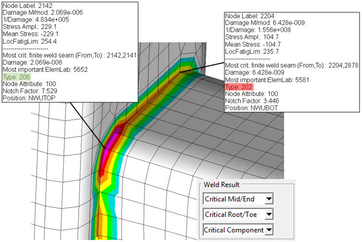

Modal stresses and transfer functions are required for a fatigue analysis in SPECTRAL.
The modal stresses (op2 format) come from an eigenfrequency analysis, the transfer functions (pch format) from a modally reduced frequency response analysis under unit loads.
By default, Optistruct also takes the residual vectors/modes into account for a frequency response analysis.
To ensure that the associated stresses are also included in the op2 file, a special parameter ("MODAL") must be specified when defining the output.
An example of a load case definition follows:
FREQ = 100
METHOD(STRUCTURE) = 101
SDAMPING(STRUCTURE) = 102
SPC = 1
$$
$$ Frequency Response Analysis
SUBCASE 1
DLOAD = 301
SDISPLACEMENT(PUNCH, SORT1) = ALL
STRESS(SORT1,OP2,MODAL)=ALL
BEGIN BULK
…
The warning indicates that the frequency range of the PSD definition is greater than that which is covered by the transfer functions. Consequently, loads are analyzed in a frequency range of the PSD for which the dynamic behavior of the structure is unknown. This warning can be ignored or modifications can be made to the input data.
But what happens if the warning is ignored?
At the basic level, a common SPECTRAL analysis is carried out. However, for those frequency ranges for which no sampling points of the transfer functions are available, the neighboring, most recently valid sampling point of the transfer function is taken and used for the additional, missing frequencies.
It is recommended to avoid this error message by modifying input data. This entails checking the PSD definition for correctness in the first step and correcting it if necessary. If it can be assumed that the PSD definition is correct, natural frequency analysis and response analysis must be carried out at least for that frequency range for which the PSD is also defined. Figure 1 clearly illustrates this situation.
A special point becomes evident in the graphic display of the equivalent stress PSD in the results evaluation if the warning is ignored: the originally defined frequency range of the transfer functions is displayed here. The PSD content from frequency ranges lying below or above this is added to the first or last sampling point, respectively.
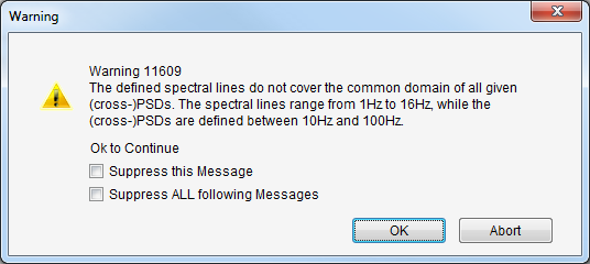
Test course distance
The test course distance is used for the recalculation of the damage for a damage value over a certain distance. This means that if the load spectrum used refers, for example, to a 5 km test course, then 5 can be entered here to calculate the damage result for a one kilometer test course. The reciprocal of the damage then provides information about how many test course kilometers can be completed until the damage value of 1 is reached. Thus, the damage result is divided by the value in the "Test Course Distance" field.
CAUTION: The scaling of the damage only takes place in the FEMFAT result file (*.dma)!
Lets assume that FEMFAT produces a damage value of 0.8 from a calculation; how should this value be interpreted? First of all a couple of details need to be cleared up. If, for example, the value has been produced at an FE-node subject to a singular load (e.g. force application, center node of a parabolic element with beam, rod or RBE connection), then this must be excluded from the usual assessment.
Suppose you need to look at an "assessable" FE-node with value D=0.8, then the material file used in FEMFAT is the point from which to proceed. The material file contains a percentage for the survival probability. This survival probability (Pü) of e.g. 97.5% (typical for most FKM materials), indicates that for the specified load, and assuming a Gaussian normal distribution, 97.5% of samples will take a larger number of load cycles before crack initiation. Remember: the S/N curves used in the FEMFAT materials are "crack initiation S/N curves".
In statistics, a Gaussian distribution is uniquely described by the mean value and the standard deviation. In the Haibach method, the ratio of the number of load cycles N90% at which 90% of the samples are cracked to N10% the number of load cycles at which only 10% of the samples are cracked, is used as the range of variation TN. The standard deviation s and the range of dispersionTN are related by the equation:
This equation is obtained because the 90% and 10% quantile for a standard normal distribution lie 1.28*s to the left and right of the mean value. FEMFAT processes the range of variation TS, which describes a similar behavior but only for the vertical direction i.e. the amplitude stresses. In the low-cycle region before the fatigue cycle limit, the two ranges are related by the gradient k of the S/N curve:

Thus a damage value of D=0.8 means that 80% of the possible load cycles up to fracture for 97.5% survival probability have been reached. In order for FEMFAT to be able to process materials with different survival probabilities, and also make predictions for a definable survival probability, the fatigue strength is corrected using the statistical influence factor. If "u" is the standardized random variable of the Gaussian normal distribution with mean value=0 and standard deviation=1, then for a material with Pü=97.5% and a selected survival probability of 99.9%, the fatigue strength is now just 90.312% of the original value (ignoring other influencing factors):
| Pü [%] | u | f (50%) | f (90%) | f (97,5%) |
|---|---|---|---|---|
| 50 | 0,0000 | 1,0000 | 1,12250 | 1,19330 |
| 90 | 1,2816 | 0,89087 | 1,00000 | 1,06308 |
| 97,5 | 1,9600 | 0,83801 | 0,94065 | 1,00000 |
| 99 | 2,3263 | 0,81079 | 0,91011 | 0,96752 |
| 99,9 | 3,0902 | 0,75682 | 0,84953 | 0,90311 |
| 99,99 | 3,7190 | 0,71511 | 0,80271 | 0,85334 |
| 99,999 | 4,2649 | 0,68076 | 0,76415 | 0,81235 |
| 99,9999 | 4,7534 | 0,65143 | 0,73123 | 0,77735 |
For endurance-limit safety factors the procedure is as follows: take a material with 90% survival probability and range of Dispersion TS =1.25 (samples have a distribution which sufficiently approximates the standard normal distribution); if the FEMFAT result now gives a safety factor SD=1.4 for constant mean stress in a FE-node, it would be theoretically possible to increase the amplitude stress by 40% or one reads from the following graph (see FEMFAT basic user manual) the increased component survival probabilities (lower failure probability), i.e. 99.99999 % - generally quite adequate for components in the automobile and passenger transport industry.
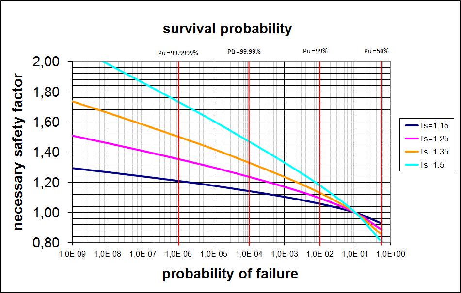
The "Results Manager" allows FEMFAT results to be scaled and combined, and the results of several analysis runs to be amalgamated to form a single result. Any number of FEMFAT results (fps files) can be imported into the "Results Manager" and combined.
Overall, there are three different options available for combining the data:
- Using the "critical" setting the respective extreme value from the main results (safety factor, damage, degree of multiaxiality,…) is exported to the result file together with the corresponding secondary results (1/safety factor, stresses, gradient,…).
- Using the "Linear" setting the values or their reciprocals are combined linearly, depending on the analysis method. The mean of the secondary results is formed using a weighting factor derived from the main results.
- Using the "Formula" setting, the FEMFAT results can be combined with great flexibility by means of a uses-defined equation. Equation input can be performed using the buttons in the menu or via the keyboard.
Example: different total damage for a Load spectra
In this case, the stresses over a crank angle of 720 degrees were analyzed by means of the dynamic simulation of a conrod. The damage at five different engine speeds (1,000 to 5,000 rpm) was combined (Figure 1) by means of modal superposition and participation factors in ChannelMAX.
Using Method 2 - "Linear", the individual partial damages arising from the various speeds can be added to a defined number of load cycles to form the overall damage:

The ensuing fps file can now be represented in VISUALIZER (Figure 2) and exported in any postprocessor Format.
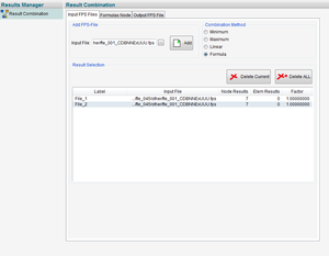
Fig. 1: "Result Manager" input
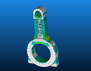
Fig. 2: Visualization of the combined results
Instead of the standard deviation s common in statistics, FEMFAT works with the load-related range of dispersion TS. The load cycle-related range of dispersion TN is determined from the load cycle number N90%, at which 90% of specimens are cracked to the load cycle number N10%, at which only 10% of samples are cracked. The following simple relationship exists between TN and TS, where k is included as the slope of the S/N curve:
TN =TkS
The range of dispersion TS can be specified for separate node groups by the user on the FEMFAT GUI. This value may vary between 1.1 and 1.6 depending on the component, material and manufacturing process. For example, in FEMFAT a value of 1.5 (after Radaj) may be specified for analyzing a welded joint in structural steel.
The default range of dispersion is defined as 1.26. This value corresponds (after Haibach) to chip-forming machining of steel components with low to medium notch effect or of notched cast iron components.
How are survival probability and failure probability related?
The figure shows the relationship between survival probability PU on the top and the failure probability PA on the bottom of the diagram for various ranges of dispersion. The diagram was compiled using the Gaussian distribution (log N) usual for FEMFAT, the rated survival probability is 90%.
One type of failure probability can be determined from
PA* = 1 - PU
where PA* represents the failure probability identified using the simplified method, because statistical data, e.g. on dispersion ranges for operating loads from several measurements, are often not available.
PA* can be used in simplification in place of the true failure probability PA if the dispersion ranges for operating loads are small compared to the dispersion ranges of dynamic strength, or the ratio of standard deviations of the normal distributions of load/strength is small. If this is not the case, the true failure probability PA* approaches the failure probability of a very unfavorable load, which is rarely achieved or exceeded. In many cases, the simplified failure probability PA* may be adopted.
The fatigue safety factor required for a durability assessment with a specified failure probability PA and range of dispersion TS can be read from the abscissa of figure 7.
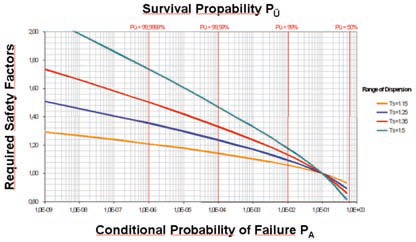
It is sometimes necessary to prepare FEMFAT results for additional postprocessors. When using the *.odb output format for the ABAQUS Viewer a small trick needs to be applied, because the FEMFAT result must always be appended to an existing *.odb file.
Procedure:
- Import the FE-structure for appending the FEMFAT result by means of the *.odb file.
- Import the *.fps file (internal FEMFAT result file, also required by FEMFAT visualizer)
- Define the *.odb output file using a new name.
- Press the "Write" button!
Using the “Results Manager” (RM), you can manage, or, more accurately, process your results from one or several FEMFAT analysis runs to form a processed results data record. Let’s assume your company policy requires the investigation of a component for several levels of a stepped load spectrum, however not with respect to the endurance limit as in FEMFAT, but instead with a 2-deflection-point S/N curve. The 2nd deflection point should be at 70% of the local endurance limit and the 2nd slope should be (2*k-1), as in Miner modified.
SOLUTION: The fps files of the damage analyses of individual collective levels are loaded in the RM and a “formula” is defined for each fps file: if( [File_1:Stress_Ampl.] < [File_1:L ocFatigLim]*0.7),0,[File_1:Damage_ M|mod])
Up to 10 results can be generated in the new fps file this way. Depending on the number of levels, you will get several such fps files which can be processed in another pass to form a single end result. The “linear combination” approach can be used here in which the individual damage results are added up weighted according to their frequency of occurrence.
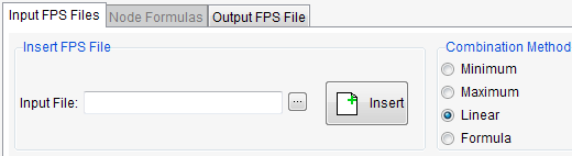
One of the numerous useful outputs of a MAX analysis is an ASCII file with the extension .rfm. It contains information about the rain-flow matrix at the critical node.However, if you open this file in an edi-tor, you will see that it contains more than just one 64x64 matrix. But let’s take one thing at a time: At the very top, you will find 2 lines with the class limits for amplitude stress and mean stress. Then there are a total of six 64x64 blocks; three each for the closed and open cycles. The first block contains the number of closed cycles and the second block contains the share (in percent) of the respective matrix entries relative to the total damage. Analogous to this, the blocks for the number of open cycles follow with their share (in percent) of the total damage. The fifth and sixth matrix contain the damage referenced to the number of cycles for the closed and open cycles. These, by the way, are also the same six matrices which you can have displayed in FEMFAT using the rainflow matrix viewer from the Visualization menu.
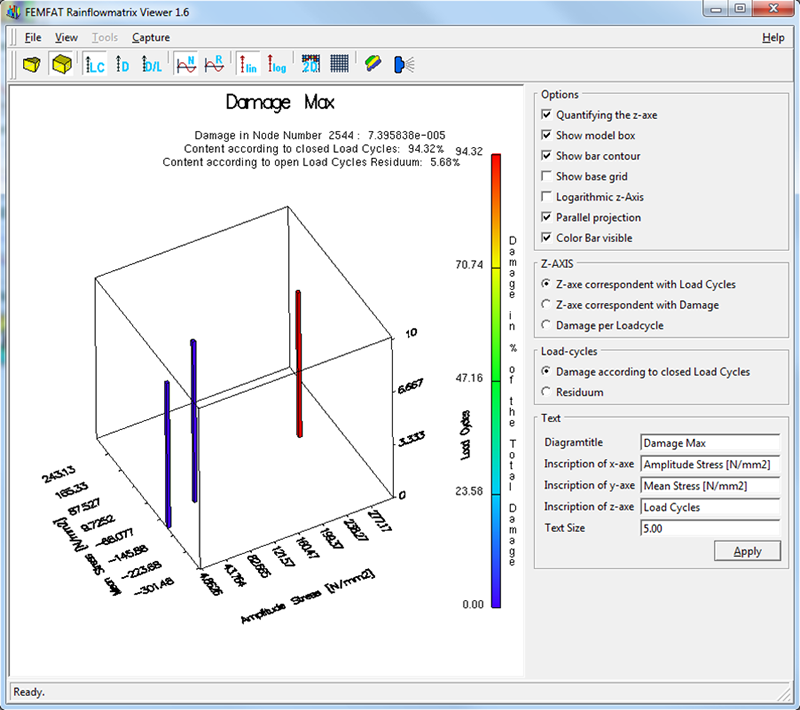
The results of a successful FEMFAT analysis are written to the binary „Permanent Scratch“ file (fps file). This file can be opened with the VISUALIZER and used for the evaluation of the fatigue results. All functionalities are available that can be expected from a modern postprocessor. Particularly profitable the VISUALIZER can be used in the interpretation of results, because all requested detail results (over 50) are available at once. Alternatively, you can export the FEMFAT results to a dma result file for other postprocessor programs. Since for most interfaces this export must take place in the form of a displacement vector, a maximum of six results are available. The selection of the desired detailed results is done in the menu „Output“ in the tab „DMA-Column Setting“ by unambiguous assignment of a column number from one to six. This selection can be made especially conveniently with a right mouse click (see figure).
Tip: The output of FEMFAT results in a dma file is also possible after completion of the FEMFAT session. All you need is the fps file with the results you would like to export. Start FEMFAT and go directly to the „Output“ menu. Use the „Import“ button there to read in the fps file. Then you can select the desired results as well as the interface and export the results by pressing the „Write“ button.
Note: the Abaqus interface requires a previous model import (odb file) from the “FE Entities” menu.